The gut-to-soil tutorial is intended to be the primary entry point for new users who are interested in working through a full analysis of microbiome data with QIIME 2, before applying it to their own data. As we progress, you can run the commands from the tutorial on your own computer and you will be presented with exercises and solutions to encourage you to explore and interpret the results of the analysis steps.
This tutorial assumes two things:
First, that you’ve read Getting Started with QIIME 2. This will help you understand some of the informatics-y jargon used here. Also, see the project glossary for help with our jargon.
And second, that you have a working installation of QIIME 2 (learn how to install QIIME 2 at https://
install .qiime2 .org). If you’d rather not install QIIME 2 before reading this document, all outputs that will be generated are linked from this document - so, the QIIME 2 installation is optional, but the tutorial is written assuming that you’re running each command (including those in the Exercises) as they are presented.
The data used in this tutorial
The original study data
The data used here was originally generated for Meilander et al. (2025): Upcycling Human Excrement: The Gut Microbiome to Soil Microbiome Axis, which profiles 15 biological replicates of mesophilic human excrement composting (HEC). The full dataset is available in a Zenodo archive Caporaso & Meilander, 2025 for continued exploration by learners.
This is 16S rRNA data generated using the Earth Microbiome Project protocol Caporaso et al., 2012. Specifically, the hypervariable region 4 (V4) of the 16S rRNA gene was amplified using the F515-R806 primers—a broad-coverage primer pair for Bacteria that also amplifies some Archaea. Paired-end sequencing was performed on an Illumina MiSeq using the 2 ✕ 250 base pair chemistry. Full details are presented in the original publication.
Samples used to generate this dataset were collected from 15 biological replicates over a 52-week composting period from 11 human participants (note that two subjects each participated three times over the course of the experiment). Each biological replicate was maintained in a separate bucket, and we therefore refer to the replicates as buckets in the original manuscript and here. Three HE samples were collected from each participant using sterile cotton swabs. Bulking material samples (1–2 per bucket, depending on the bulking materials used) were collected before composting. Environmental samples included swabs of the area surrounding each composting toilet, the interior surface of each toilet chamber prior to use, and the interior surface of each composting bucket before material was added. Weekly samples were then collected from each bucket for 52 weeks (composting timepoints 1–52). Food and landscape waste compost (FLWC) samples were collected from a composting facility at Northern Arizona University, six small agricultural farms, and two backyard gardens in Flagstaff, Arizona. These samples represented compost produced from pre- and post-consumer food waste co-composted with landscape materials, including leaves, pine needles, branches, and straw. In addition, sequencing data from 41 soil samples from the Earth Microbiome Project (EMP) “EMP500” were obtained from publicly available Qiita data (study 13114) and used in a pooled analysis (i.e., not resequenced for this project). Together the FLWC and soil samples served as reference samples.
The data subset for the hands-on tutorial
The data used here is a subset (a single sequencing run) of the Meilander et al. (2025) data, specifically selected so that this tutorial can be run quickly on a personal computer. This subset contains 104 samples with data from 13 buckets and includes 25 HEC samples, 19 HE samples, 20 FLWC samples, 15 Bulking Material samples, 10 samples from inside toilets pre-use, 10 soil samples collected near the composting toilets, and various additional control samples. This was a test sequencing run performed while sample collection was ongoing, and was intended to cover the different sample types that had been collected (e.g., to detect issues with extraction or sequencing protocols). As such, most buckets don’t have dense temporal information but Bucket 5 is the exception with 14 samples over the first 18 weeks of composting. We therefore primarily focus on the cross-sectional aspects of data analysis in this tutorial, though you can visualize the time series in Bucket 5 with this subset; future longitudinal tutorials will be developed on different subsets of this study data and from metagenomic and metatranscriptomic data generated in ongoing HEC projects. No EMP500 soils are used in this tutorial, so the FLWC (referred to as “Food Compost” in the study metadata) samples will serve as the reference samples here.
Constructed data for figures
In addition to the tutorial data, beginning with Figure 3 we’ll follow a constructed example dataset through the analysis to enable visualization of microbiome data as it progresses through the workflow that we’re illustrating. This constructed dataset does not represent real samples, but it is inspired by the tutorial data. Specifically it models seven samples: one HE sample, five HEC samples from five different timepoints over one year of composting from a single bucket, and one food compost sample. This constructed dataset is intended to provide a way for readers to visualize and assess their understanding of the analysis process as we progress through the tutorial in a way that would be impossible even on the relatively simple tutorial data.
Installing QIIME 2
Install QIIME 2 by following the installation documentation. The screenshots presented in this section were taken against the JupyterLab environment in the QIIME 2 2026.7 workshop Docker container. You can use that, or any way of installing QIIME 2 that is covered in the documentation.
After loading your QIIME 2 environment - either by calling conda activate ..., through Docker, or through any other supported approach, in a terminal, type qiime info, and press return.
The result should look like that in the command terminal of Figure 1.
(Note that the file browser side bar will only be there if you’re working in JupyterLab.)
If you received errors with these steps, we recommend looking for similar posts on the QIIME 2 Forum, and posting yourself if you don’t find relevant troubleshooting information.
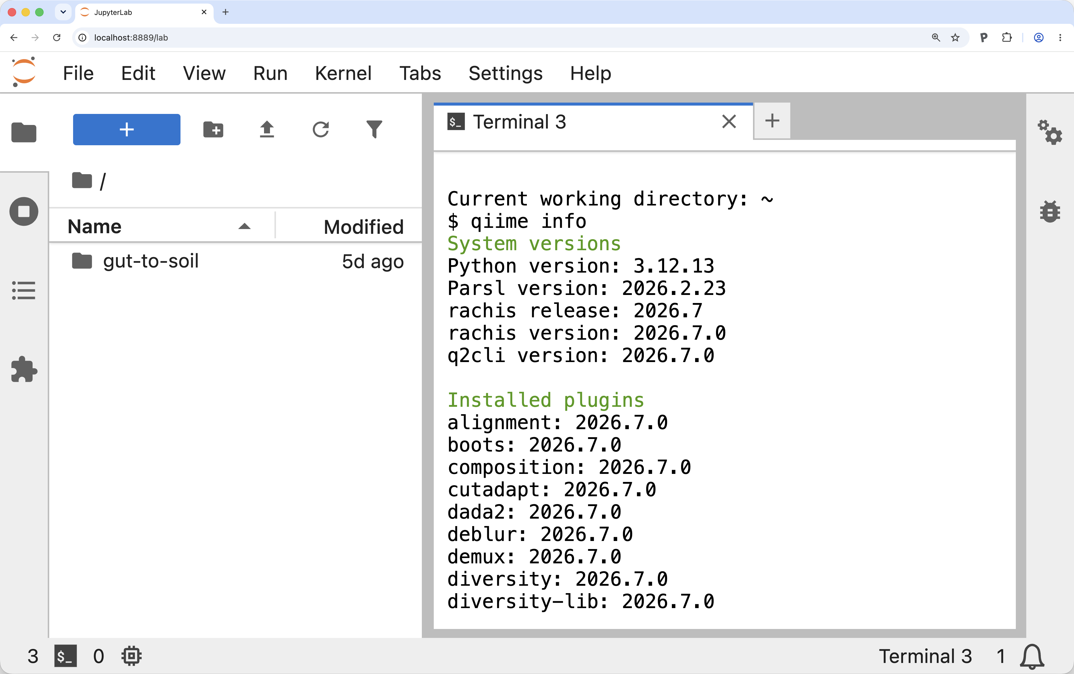
Figure 1:QIIME 2 2026.7 workshop Docker container. Example of the view after running qiime info in the QIIME 2 2026.7 workshop Docker container. After launching the workshop container and running qiime info, if your display looks like this you should be safe to continue with the tutorial.
Reviewing sample metadata and running a QIIME 2 command
Before starting the analysis, we’ll explore the sample metadata to get familiarized with the samples used in this study.
Sample metadata generally contains per-sample information relevant to your study.
In this tutorial, the sample metadata includes information such as the sample type (see the SampleType column), the sample’s pH at time of collection (see the Compost pH column), which of our biological replicates it came from (see the Bucket column), which composting timepoint the sample came from (if relevant, see the Composting Time Point column), and more.
To learn about metadata in QIIME 2, including how it should be formatted, refer to our documentation on the metadata format.
First, create a directory to work on this tutorial in and then change into that directory.
mkdir gut-to-soil/
cd gut-to-soil/
Run the following command to download the sample metadata as tab-separated text from Zenodo and save it in the file sample-metadata.tsv.
This sample-metadata.tsv file is used throughout the rest of the tutorial.
wget -O 'sample-metadata.tsv' \
  'https://gut-to-soil-tutorial.readthedocs.io/en/latest/data/gut-to-soil/sample-metadata.tsv'
from qiime2 import Metadata
from urllib import request

url = 'https://gut-to-soil-tutorial.readthedocs.io/en/latest/data/gut-to-soil/sample-metadata.tsv'
fn = 'sample-metadata.tsv'
request.urlretrieve(url, fn)
sample_metadata_md = Metadata.load(fn)
library(reticulate)

Metadata <- import("qiime2")$Metadata
request <- import("urllib")$request

url <- 'https://gut-to-soil-tutorial.readthedocs.io/en/latest/data/gut-to-soil/sample-metadata.tsv'
fn <- 'sample-metadata.tsv'
request$urlretrieve(url, fn)
sample_metadata_md <- Metadata$load(fn)
sample_metadata = use.init_metadata_from_url(
   'sample-metadata',
'https://zenodo.org/records/15390940/files/gut-to-soil-tutorial-sample-metadata.tsv?download=1')sample-metadata.tsv| download
QIIME 2’s q2-metadata plugin provides a Visualizer called tabulate that generates a convenient view of a sample metadata file.
Run the following command, which is the first QIIME 2 command that you should run in this tutorial:
qiime metadata tabulate \
  --m-input-file sample-metadata.tsv \
  --o-visualization sample-metadata.qzv
import rachis.plugins.metadata.actions as metadata_actions
sample_metadata_viz, = metadata_actions.tabulate(
input=sample_metadata_md,
)metadata_actions <- import("rachis.plugins.metadata.actions")
action_results <- metadata_actions$tabulate(
input=sample_metadata_md,
)
sample_metadata_viz <- action_results$visualizationuse.action(
use.UsageAction(plugin_id='metadata',
action_id='tabulate'),
use.UsageInputs(input=sample_metadata),
use.UsageOutputNames(visualization='sample_metadata')
)This will generate a QIIME 2 Visualization.
Figure 2 shows this Visualization viewed inside the QIIME 2 2026.7 workshop Docker container.
Visualizations can also be viewed by loading them with rachis-view - navigate to rachis-view in a web browser, and drag and drop the sample-metadata.qzv file.
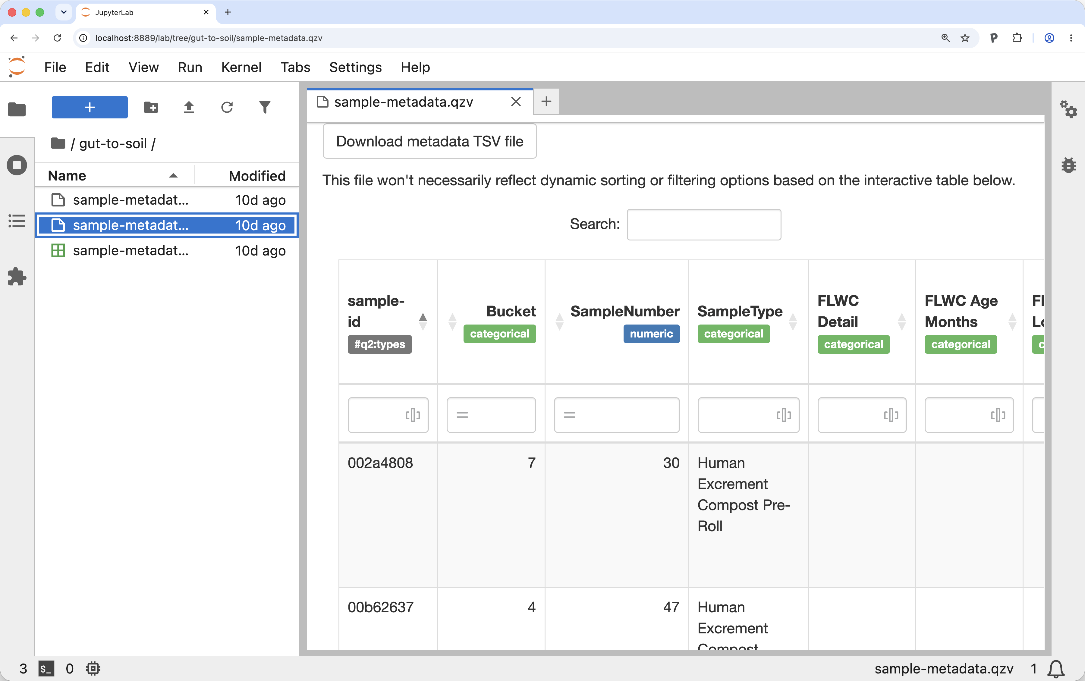
Figure 2:A view of the sample metadata in a QIIME 2 Visualization. Example of the view after running qiime metadata tabulate on the gut-to-soil tutorial metadata in the QIIME 2 2026.7 workshop Docker container. Running qiime metadata tabulate on your metadata and viewing the result is a good way to review your metadata as QIIME 2 sees it.
Figure 3 presents a view of sample metadata for the constructed dataset described above. These samples are not real, but rather represent a few samples that we’ll use in the figures throughout the tutorial to assist readers with visualizing the data we are working with. In your interactive tabulated view of the metadata, explore the metadata columns that are presented in Figure 3.

Figure 3:Simplified view of sample metadata for a few samples in the constructed data. Sample metadata for the constructed data set used in the manuscript figures. Throughout the figures in this manuscript, we’ll follow a constructed, illustrative set of samples through data analysis. These are the metadata that describe these samples. In general, metadata is provided in .tsv files. Notice that there are three color-coded sample types: Human Excrement (orange), Human Excrement Compost (blue, with lightness correlated with the Composting Time Point), and Food Compost (green). The first six samples are associated with a single biological replicate called Bucket 42, and the final sample is not associated with a biological replicate. Because the “Bucket” column does not have an applicable value for sample d419, that cell is left blank per the rachis metadata standard for representing missing or inapplicable metadata.
Access already-imported QIIME 2 data
This tutorial begins with paired-end read sequencing data generated on an Illumina MiSeq that has already been demultiplexed and imported into a QIIME 2 Artifact. You can access this data by running the following command:
wget -O 'demux.qza' \
  'https://gut-to-soil-tutorial.readthedocs.io/en/latest/data/gut-to-soil/demux.qza'
from qiime2 import Artifact

url = 'https://gut-to-soil-tutorial.readthedocs.io/en/latest/data/gut-to-soil/demux.qza'
fn = 'demux.qza'
request.urlretrieve(url, fn)
demux = Artifact.load(fn)
Artifact <- import("qiime2")$Artifact

url <- 'https://gut-to-soil-tutorial.readthedocs.io/en/latest/data/gut-to-soil/demux.qza'
fn <- 'demux.qza'
request$urlretrieve(url, fn)
demux <- Artifact$load(fn)
demux = use.init_artifact_from_url(
   'demux',
'https://zenodo.org/records/15390940/files/gut-to-soil-tutorial-nano2-demux-10p.qza?download=1')Demultiplexed sequence data is data where sequences have already been assigned to the sample that they were observed in. Paired-end read data means that for every sequence read in your dataset you have a forward read (which typically starts from the 5’ end of the target amplicon sequence) and a reverse read (which typically starts from the 3’ end of the targeted amplicon). In demultiplexed paired-end read data, you’ll generally start with two fastq files per sample, one for the forward read, and one for the reverse read. For QIIME 2 to work with these data, it needs to know which of your fastq files contains the forward reads and which contains the reverse reads for each sample. For importing these data into QIIME 2, we generally recommend the use of a fastq manifest file which maps the sample identifier to the forward and reverse read file paths. Figure 4 presents an illustration of a fastq manifest file alongside two example fastq files. Like in Figure 3, these are not real data but rather the constructed dataset generated for illustrative purposes.
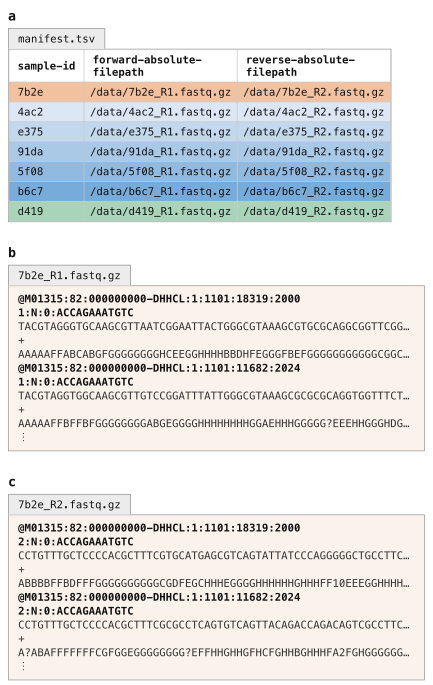
Figure 4:Schematic view of a fastq manifest file and demultiplexed fastq data, ready for import into QIIME 2. In general, demultiplexed Illumina sequencing data is stored in a pair of files per sample corresponding to the forward and reverse reads. A fastq manifest file (panel a) is a sample metadata file with three specific columns that link specific samples to the absolute file paths where their forward and reverse reads can be found. Fastq files for one sample are illustrated here: panels b and c are the forward and reverse reads for sample 7b2e. It is common for the sample ids to be embedded in the fastq file names (as is illustrated here) but that is not a requirement for QIIME 2. Rather, the file names can be anything, and the manifest file links the files to the samples.
Notice the similarity of the fastq manifest in Figure 4 and the sample metadata in Figure 3.
A fastq manifest is a specific type of sample metadata file.
Specifically, it’s one that contains forward-absolute-filepath and reverse-absolute-filepath columns, with absolute file paths present for every sample identifier in the table.
Because sequence data can be delivered to you in many different forms, it’s not possible to cover the varieties here. Instead, we refer you to How to import data for use with QIIME 2 to learn how to import your data. If you want to learn why importing is necessary, refer to Why importing is necessary.
To simplify processing of your data, we recommend that you ask your sequencing center to provide data already demultiplexed. This should be something they can easily do, and it simplifies processing as you don’t need to know how data was barcoded for multiplexed sequencing. You can also ask them to provide a fastq manifest file for your sequencing data, which should be easy for them to generate based on the file specification; if they’re not able to do this, you can use a tool like fq-manifestor to generate one.
Summarize demultiplexed sequences
When you have demultiplexed sequence data, the next step is typically to generate a visual summary of it.
This allows you to determine how many sequences were obtained per sample, and also to get a summary of the distribution of sequence quality at each position in your sequence data.
Run the following command to generate an interactive quality plot Visualization.
Load the visualization (for example, by using rachis-view).
qiime demux summarize \
  --i-data demux.qza \
  --o-visualization demux.qzv
import rachis.plugins.demux.actions as demux_actions
demux_viz, = demux_actions.summarize(
data=demux,
)demux_actions <- import("rachis.plugins.demux.actions")
action_results <- demux_actions$summarize(
data=demux,
)
demux_viz <- action_results$visualizationuse.action(
use.UsageAction(plugin_id='demux',
action_id='summarize'),
use.UsageInputs(data=demux),
use.UsageOutputNames(visualization='demux'))Solution to Exercise 1
There are 104 samples represented in this sequencing data, and the median sequencing depth (number of sequences per sample) is 659.5. The median quality score at position 200 in the forward reads is 37.
Trimming of PCR primers
The protocol used for sequencing of these data results in sequences that do not include the PCR primers at the beginning and end of the reads. This is not always the case however: sometimes you will want to remove primers before proceeding to the next step. If the primers are definitely present and of known length, this can be done with q2-dada2 during sequence quality control, which will be covered next; if the primers are not at a known position, of variable length, or may or may not be present (e.g., when running a meta-analysis), you can use QIIME 2’s cutadapt plugin.
Sequence quality control and feature table construction
QIIME 2 plugins are available for several quality control methods, including DADA2 Callahan et al., 2016, Deblur Amir et al., 2017, and basic quality-score-based filtering Bokulich et al., 2013. In this tutorial, we present this step using DADA2, which integrates quality control with the definition of the “features” that will be used to describe our samples.
The primary results of interest from our DADA2 step will be a FeatureTable[Frequency] QIIME 2 artifact, which contains counts (frequencies) of each amplicon sequence variant (ASV, or unique sequence post-quality-control) in each sample in the dataset, and a FeatureData[Sequence] QIIME 2 artifact, which maps feature identifiers in the FeatureTable to the sequences they represent.
Illustrative examples of these two outputs are presented in Figure 5.
Notice that the column headers in the FeatureTable[Frequency] map directly onto the sequence identifiers in the FeatureData[Sequence].
These are the feature identifiers.
In some cases, feature identifiers can be related across analyses, and in some cases they cannot be.
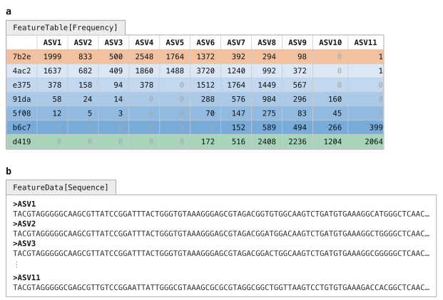
Figure 5:A feature table and the corresponding feature sequences. A FeatureTable[Frequency] (panel a) describes how many times each feature was observed in each sample. In this feature table, the features are amplicon sequence variants, and each ASV’s sequence is stored in the corresponding FeatureData[Sequence] artifact (panel b). The rows in this feature table represent the samples and the columns represent the features.
DADA2 is a pipeline for detecting and correcting (where possible) errors in Illumina amplicon sequence data. As implemented in the q2-dada2 plugin, this quality control process will additionally filter any phiX reads (commonly present in marker gene Illumina sequence data to diversify the base calls at each position) that are identified in the sequencing data, filter chimeric sequences, and merge paired-end reads.
The denoise-paired action, which we’ll use here, requires you to provide values for four parameters that are used in quality filtering:
trim-left-f <a>, which trims off the first<a>bases of each forward readtrim-left-r <b>, which trims off the first<b>bases of each reverse readtrunc-len-f <c>, which truncates each forward read at position<c>trunc-len-r <d>, which truncates each reverse read at position<d>
These parameters allow the user to remove low-quality regions of the sequences from the beginning and end of the sequences.
To determine what values to pass for these parameters, review the Interactive Quality Plot tab in the demux.qzv file that was generated above.
Solution to Exercise 2
The answer to this question is subjective, and something you’ll need to determine on your own. When I review this, I notice that the quality of the initial bases seems to be high, so I choose not to trim any bases from the beginning of the sequences. The quality also seems good all the way out to the end, though maybe dropping off after 250 bases. I’ll therefore truncate at 250. I’ll keep these values the same for both the forward and reverse reads, though that is not a requirement. These decisions correspond to the following parameter settings:
trim-left-f: 0trim-left-r: 0trunc-len-f: 250trunc-len-r: 250
Now run the following DADA2 command. This step may take up to 10 minutes to complete—it’s the longest-running step in this tutorial.
qiime dada2 denoise-paired \
  --i-demultiplexed-seqs demux.qza \
  --p-trim-left-f 0 \
  --p-trunc-len-f 250 \
  --p-trim-left-r 0 \
  --p-trunc-len-r 250 \
  --o-representative-sequences asv-seqs.qza \
  --o-table asv-table.qza \
  --o-denoising-stats denoising-stats.qza \
  --o-base-transition-stats base-transition-stats.qza
import rachis.plugins.dada2.actions as dada2_actions
asv_table, asv_seqs, denoising_stats, base_transition_stats = dada2_actions.denoise_paired(
demultiplexed_seqs=demux,
trim_left_f=0,
trunc_len_f=250,
trim_left_r=0,
trunc_len_r=250,
)dada2_actions <- import("rachis.plugins.dada2.actions")
action_results <- dada2_actions$denoise_paired(
demultiplexed_seqs=demux,
trim_left_f=0L,
trunc_len_f=250L,
trim_left_r=0L,
trunc_len_r=250L,
)
asv_seqs <- action_results$representative_sequences
asv_table <- action_results$table
denoising_stats <- action_results$denoising_stats
base_transition_stats <- action_results$base_transition_statsasv_seqs, asv_table, denoising_stats, base_transition_stats = use.action(
use.UsageAction(plugin_id='dada2',
action_id='denoise_paired'),
use.UsageInputs(demultiplexed_seqs=demux,
trim_left_f=0,
trunc_len_f=250,
trim_left_r=0,
trunc_len_r=250),
use.UsageOutputNames(representative_sequences='asv_seqs',
table='asv_table',
denoising_stats='denoising_stats',
base_transition_stats='base_transition_stats'))asv-seqs.qza| download | viewasv-table.qza| download | viewdenoising-stats.qza| download | viewbase-transition-stats.qza| download | view
One of the outputs created by DADA2, denoising-stats, is a summary of the denoising run.
That is generated as an Artifact, so it can’t be viewed directly.
However, this is one of many rachis types that can be viewed as Metadata—a very powerful concept that we’ll use again later in this tutorial.
Learning to view artifacts as Metadata creates nearly infinite possibilities for how you can explore your microbiome data with QIIME 2.
To do this, we’ll again use the q2-metadata plugin’s tabulate visualizer, but this time we’ll apply it to the DADA2 statistics.
qiime metadata tabulate \
  --m-input-file denoising-stats.qza \
  --o-visualization denoising-stats.qzv
from rachis import Metadata
stats_as_md_md = denoising_stats.view(Metadata)
denoising_stats_viz, = metadata_actions.tabulate(
input=stats_as_md_md,
)stats_as_md_md <- denoising_stats$view(Metadata)
action_results <- metadata_actions$tabulate(
input=stats_as_md_md,
)
denoising_stats_viz <- action_results$visualizationstats_as_md = use.view_as_metadata('stats_as_md', denoising_stats)
use.action(
use.UsageAction(plugin_id='metadata',
action_id='tabulate'),
use.UsageInputs(input=stats_as_md),
use.UsageOutputNames(visualization='denoising_stats'))Solution to Exercise 3
The samples with identifiers 21f2e6d0, 9d3aefae, and 27c41e29 had the lowest percentage of input reads passing the quality filter.
(Sample 48dff3fa had zero input reads.)
21f2e6d0 is a human excrement compost (HEC) sample from Bucket 11 and Composting Time Point 28.
9d3aefae is a human excrement (HE) sample, also from Bucket 11.
27c41e29 is a sample of Soil Nearby the Toilet for Bucket 12.
48dff3fa is a Bulking Material sample for Bucket 7.
Solution to Exercise 4
qiime metadata tabulate \
  --m-input-file sample-metadata.tsv denoising-stats.qza \
  --o-visualization sample-metadata-w-dada2-stats.qzv
sample_metadata_and_dada2_stats_md_md = sample_metadata_md.merge(stats_as_md_md)
sample_metadata_w_dada2_stats_viz, = metadata_actions.tabulate(
input=sample_metadata_and_dada2_stats_md_md,
)sample_metadata_and_dada2_stats_md_md <- sample_metadata_md$merge(stats_as_md_md)
action_results <- metadata_actions$tabulate(
input=sample_metadata_and_dada2_stats_md_md,
)
sample_metadata_w_dada2_stats_viz <- action_results$visualizationsample_metadata_and_dada2_stats_md = use.merge_metadata('sample_metadata_and_dada2_stats_md', sample_metadata, stats_as_md)
use.action(
use.UsageAction(plugin_id='metadata',
action_id='tabulate'),
use.UsageInputs(input=sample_metadata_and_dada2_stats_md),
use.UsageOutputNames(visualization='sample_metadata_w_dada2_stats'))Feature table and feature data summaries
After DADA2 completes, you’ll want to explore the resulting data.
You can do this using the following two commands, which will create visual summaries of the data.
The feature-table summarize action will give you information on how many sequences are associated with each sample and with each feature, histograms of those distributions, and some related summary statistics.
qiime feature-table summarize \
  --i-table asv-table.qza \
  --m-metadata-file sample-metadata.tsv \
  --o-summary asv-table.qzv \
  --o-sample-frequencies sample-frequencies.qza \
  --o-feature-frequencies asv-frequencies.qza
import rachis.plugins.feature_table.actions as feature_table_actions
asv_frequencies, sample_frequencies, asv_table_viz = feature_table_actions.summarize(
table=asv_table,
metadata=sample_metadata_md,
)feature_table_actions <- import("rachis.plugins.feature_table.actions")
action_results <- feature_table_actions$summarize(
table=asv_table,
metadata=sample_metadata_md,
)
asv_table_viz <- action_results$summary
sample_frequencies <- action_results$sample_frequencies
asv_frequencies <- action_results$feature_frequencies_, _, asv_frequencies = use.action(
use.UsageAction(plugin_id='feature_table',
action_id='summarize'),
use.UsageInputs(table=asv_table,
metadata=sample_metadata),
use.UsageOutputNames(summary='asv_table',
sample_frequencies='sample_frequencies',
feature_frequencies='asv_frequencies'))asv-table.qzv| download | viewsample-frequencies.qza| download | viewasv-frequencies.qza| download | view
Two additional output artifacts are generated here, and the contents of these are illustrated in Figure 6.
The Sample Frequencies table presents the total sequence count (Frequency) and the number of features with a count greater than zero in each sample.
The Feature Frequencies table presents the total number of sequences observed for each feature, and number of samples that each feature was observed in.
The summarize action that we’re using here is a Pipeline; recall that Pipelines only generate Artifacts and/or Visualizations as output.
Notice that the structure of the Sample Frequencies table is the same as our sample metadata in Figure 3.
This artifact is in fact a metadata file, but in Artifact form—the semantic type used here is ImmutableMetadata, which should be interpreted as metadata inside of an Artifact.
An ImmutableMetadata Artifact can be provided anywhere metadata is required in QIIME 2, or can be exported to a .tsv file.
The Feature Frequencies table is also an example of an ImmutableMetadata Artifact, but in this case it contains feature metadata instead of sample metadata.
The format and use of sample and feature metadata is identical, but you can think of them as describing the entities represented on the opposing axes in the table.
Sample and feature metadata are powerful concepts in the rachis ecosystem—understanding these, and how they are used, opens many opportunities for different types of analyses.
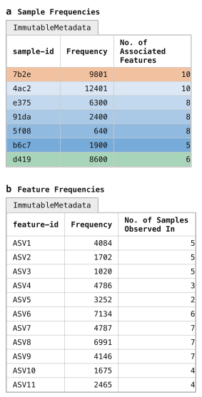
Figure 6:Per-sample and per-feature summaries of the feature table. Sample frequency summaries (panel a) and feature frequency summaries (panel b) are generated as output of qiime feature-table summarize. Notice that these are formatted a lot like metadata. This is not a coincidence, but rather these artifacts are of artifact class ImmutableMetadata, which is the class for metadata that is stored in Artifacts. These can be provided as-is as input anywhere that metadata is used, and they can be exported to .tsv files if needed by calling qiime tools export. By design, rachis commands only generate Results as output so data provenance can be embedded in all outputs. The ImmutableMetadata artifact class is used by rachis commands to output metadata as needed.
Panel a represents sample metadata, while panel b represents feature metadata.
Solution to Exercise 5
There are 39,949 total sequences represented in this feature table.
The identifier of the feature observed the largest number of times is c6c3ab4e828fb40d6e05967b7aac9338.
Its sequence was observed 1,334 times across 23 samples.
The feature-table tabulate-seqs action will provide a mapping of feature IDs to sequences, and provide links to easily BLAST each sequence against the NCBI nt database.
We can also include the feature frequency information in this visualization by passing it as metadata, similar to how we merged metadata in Exercise 4.
In this case, however, we’re looking at feature metadata, as opposed to sample metadata.
As far as QIIME 2 is concerned, there is no difference between these two—in our case, it’ll only be the identifiers that differ.
This visualization will be very useful later in the tutorial when you want to learn more about important specific features in the dataset.
qiime feature-table tabulate-seqs \
  --i-data asv-seqs.qza \
  --m-metadata-file asv-frequencies.qza \
  --o-visualization asv-seqs.qzv
asv_frequencies_md_md = asv_frequencies.view(Metadata)
asv_seqs_viz, = feature_table_actions.tabulate_seqs(
data=asv_seqs,
metadata=asv_frequencies_md_md,
)asv_frequencies_md_md <- asv_frequencies$view(Metadata)
action_results <- feature_table_actions$tabulate_seqs(
data=asv_seqs,
metadata=asv_frequencies_md_md,
)
asv_seqs_viz <- action_results$visualizationasv_frequencies_as_md = use.view_as_metadata('asv_frequencies_md',
asv_frequencies)
use.action(
use.UsageAction(plugin_id='feature_table',
action_id='tabulate_seqs'),
use.UsageInputs(data=asv_seqs,
metadata=asv_frequencies_as_md),
use.UsageOutputNames(visualization='asv_seqs'),
)Solution to Exercise 6
There are many equivalently high scoring BLAST hits for this ASV sequence (100% match covering 100% of the query sequence), and the GenBank records for many of the hits suggest it’s an organism associated with the human gut microbiome. The first result returned (as of this writing on 28 August 2026; GenBank: FJ368087.1) labels this as a 16S rRNA sequence from an Uncultured bacterium clone and notes that it was identified in human fecal samples. Other BLAST hits suggest that it’s a member of the Blautia genus. Conflicting species labels, including luti and wexlerae, are associated with top scoring BLAST results, suggesting that we likely don’t have species resolution for this short 16S sequence.
Clustering ASVs into Operational Taxonomic Units (OTUs)
OTU clustering was historically done as a crude quality control step (i.e., assuming that slight differences were a result of sequencing error, not true biological variation) and to speed up processing of data when the software and computers we were using for these analyses were less capable. This would generally be based on grouping sequences based on their percent identity to one another; for example, if two ASVs’ sequences matched each other at ≥ 97% identity, they would be represented in the feature table as a single feature with their counts summed together. However, we now have much better quality control methods, and more capable computers, and, as a result, OTU clustering is no longer considered best practice. We don’t recommend OTU clustering in most workflows, nor do we apply it in the gut-to-soil tutorial.
We instead recommend ASVs as features in marker gene studies because they provide higher resolution, improve reproducibility, and facilitate more accurate taxonomic classification. Because ASVs represent exact amplicon sequences, they can be consistently identified across samples and datasets and facilitate comparisons across microbiome studies.
It is however possible to do OTU clustering with QIIME 2, and you can find instructions in our documentation if you’d like to do this. Figure 7 illustrates how the ASVs in the example data might be grouped into OTUs. Notice that the resolution of the resulting feature table is lower: ASVs 9 and 10, for example, are grouped into OTU7, and that masks the observation that ASV10 is absent from several of the earlier samples in our time series. This may therefore be masking useful information that could have been lost from our study.

Figure 7:Clustering ASVs into OTUs. Our ASV-based feature table (panel a) could be clustered into an OTU-based feature table (panel b), based on the similarity of the ASV sequences (Figure 5b). In our constructed data, if our ASV sequences are clustered at 90% identity using qiime vsearch cluster-features-de-novo, ASVs 1–3 collapse into OTU1, and ASVs 9–10 collapse into OTU7. During that collapsing, the ASV counts are summed such that the OTU count is equal to the sum of the counts of the ASVs it contains. The difference in these tables illustrates how OTU clustering reduces the resolution of our feature table. In general, we don’t recommend OTU clustering workflows for this reason.
Filtering features from a feature table
If you review the tabulated feature sequences or the feature detail table of the feature table summary in asv-table.qzv, which present the same data illustrated in Figure 6, you’ll notice that there are many sequences that are observed in only a single sample.
Here we’ll filter those out to reduce the number of sequences we’re working with.
When working with large feature tables, this filtering step can dramatically reduce memory (RAM) requirements for analyses that load the feature table into memory.
This can be particularly helpful when computing kmer-based diversity metrics, which we’ll get to later in this tutorial.
This filtering step will also speed up processes that operate on each feature in the feature table (such as taxonomic annotation).
This is a two-step process. First, we filter our feature table, and then we use the new feature table to filter our sequences to only the ones that are contained in the new table.
qiime feature-table filter-features \
  --i-table asv-table.qza \
  --p-min-samples 2 \
  --o-filtered-table asv-table-ms2.qza
asv_table_ms2, = feature_table_actions.filter_features(
table=asv_table,
min_samples=2,
)action_results <- feature_table_actions$filter_features(
table=asv_table,
min_samples=2L,
)
asv_table_ms2 <- action_results$filtered_tableasv_table_ms2, = use.action(
use.UsageAction(plugin_id='feature_table',
action_id='filter_features'),
use.UsageInputs(table=asv_table,
min_samples=2),
use.UsageOutputNames(filtered_table='asv_table_ms2'),
)qiime feature-table filter-seqs \
--i-data asv-seqs.qza \
--i-table asv-table-ms2.qza \
--o-filtered-data asv-seqs-ms2.qzaasv_seqs_ms2, = feature_table_actions.filter_seqs(
data=asv_seqs,
table=asv_table_ms2,
)action_results <- feature_table_actions$filter_seqs(
data=asv_seqs,
table=asv_table_ms2,
)
asv_seqs_ms2 <- action_results$filtered_dataasv_seqs_ms2, = use.action(
use.UsageAction(plugin_id='feature_table',
action_id='filter_seqs'),
use.UsageInputs(data=asv_seqs,
table=asv_table_ms2),
use.UsageOutputNames(filtered_data='asv_seqs_ms2'),
)You may notice that -ms2 is included in the new output names here.
This was added to remind us that these data artifacts are filtered to contain only those features present in a minimum of 2 samples.
Generally speaking, file names are a convenient place to store information like this, but they’re unreliable.
File names can easily be changed, and therefore could be modified to contain inaccurate information about the data they contain.
Luckily, rachis’s provenance tracking system records all of the information that we need about how results were generated.
We’re therefore free to include information like this in file names if it’s helpful for us, but we shouldn’t ever rely solely on the file names.
If you’re ever in doubt about how an Artifact or Visualization was produced, refer to rachis’s data provenance which is the definitive source of truth about how a Result was created.
Solution to Exercise 7
qiime feature-table summarize \
  --i-table asv-table-ms2.qza \
  --m-metadata-file sample-metadata.tsv \
  --o-summary asv-table-ms2.qzv \
  --o-sample-frequencies sample-frequencies-ms2.qza \
  --o-feature-frequencies asv-frequencies-ms2.qza
asv_frequencies_ms2, sample_frequencies_ms2, asv_table_ms2_viz = feature_table_actions.summarize(
table=asv_table_ms2,
metadata=sample_metadata_md,
)action_results <- feature_table_actions$summarize(
table=asv_table_ms2,
metadata=sample_metadata_md,
)
asv_table_ms2_viz <- action_results$summary
sample_frequencies_ms2 <- action_results$sample_frequencies
asv_frequencies_ms2 <- action_results$feature_frequencies_, _, asv_frequencies_ms2 = use.action(
use.UsageAction(plugin_id='feature_table',
action_id='summarize'),
use.UsageInputs(table=asv_table_ms2,
metadata=sample_metadata),
use.UsageOutputNames(summary='asv_table_ms2',
sample_frequencies='sample_frequencies_ms2',
feature_frequencies='asv_frequencies_ms2'))asv-table-ms2.qzv| download | viewsample-frequencies-ms2.qza| download | viewasv-frequencies-ms2.qza| download | view
Be sure to run this as we’re going to use one of the results below.
Taxonomic annotation
Before we begin analyzing our feature table, we’ll generate taxonomic annotations for our sequences using the q2-feature-classifier plugin Bokulich et al., 2018. We’re going to do this here by training a machine learning classifier, and then applying it to our data.
Training a taxonomic classifier
Training a machine learning based taxonomic classifier in QIIME 2 requires two artifacts as input: reference sequences (in a FeatureData[Sequence] artifact; see Figure 8a), and reference taxonomy for each of those sequences (in a FeatureData[Taxonomy] artifact; see Figure 8b).
The result of this process is a TaxonomicClassifier artifact (Figure 8c).

Figure 8:A reference database is used to train a taxonomic classifier. Machine-learning-based taxonomic classification in QIIME 2 requires two inputs: reference sequences in a FeatureData[Sequence] artifact (panel a), and taxonomic labels for the reference sequences in a FeatureData[Taxonomy] artifact (panel b). The RESCRIPt plugin can help you obtain these artifacts and prepare them for training a classifier. These are used to build a TaxonomicClassifier artifact (panel c), which is different from any artifacts that we’ve worked with to this point: rather than containing static data, it contains executable software, and that is indicated by the gear icon here.
In this illustration, the taxonomic labels are obtained from Genome Taxonomy Database (GTDB) version 232.0, while in the tutorial we work with GTDB version 202.0. GTDB version 202.0 is an older database version that is helpful for allowing the tutorial to be run on diverse computer hardware; GTDB version 232.0 is current as of this writing. The reference artifacts and the pre-trained classifier for GTDB version 232.0 are distributed at Caporaso (2026).
The taxonomic classifier used here is trained on reference sequences and taxonomy from GTDB version 202.0, which is an old version of the GTDB reference database Parks et al., 2021. We use it here because the reference data is relatively small, enabling classifier training and application to run on most modern computers. For comparison, GTDB version 202.0 contains 32,884 sequences (31,319 Bacteria + 1,565 Archaea) while GTDB version 232.0 (the most recent version, as of this writing on 2 October 2026) contains 93,770 sequences (88,481 Bacteria + 5,289 Archaea).
Training a taxonomy classifier can be a slow and memory-intensive step, and this is one of the slower steps in this tutorial.
First, we’ll obtain the sequence data and the associated taxonomy annotations.
This is done using the RESCRIPt plugin Robeson et al., 2021, which provides many utilities that are useful for training taxonomy classifiers.
Here we’ll use the get-gtdb-data action, which automates the downloading of reference data from the GTDB database.
We’ll apply it here to download the 16S reference from GTDB version 202.0, including both the FeatureData[Sequence] and FeatureData[Taxonomy] artifacts.
qiime rescript get-gtdb-data \
  --p-version 202.0 \
  --p-db-type SpeciesReps \
  --p-db-url australia \
  --o-gtdb-taxonomy reference-taxonomy.qza \
  --o-gtdb-sequences reference-sequences.qza
import rachis.plugins.rescript.actions as rescript_actions
reference_taxonomy, reference_sequences = rescript_actions.get_gtdb_data(
version='202.0',
db_type='SpeciesReps',
db_url='australia',
)rescript_actions <- import("rachis.plugins.rescript.actions")
action_results <- rescript_actions$get_gtdb_data(
version='202.0',
db_type='SpeciesReps',
db_url='australia',
)
reference_taxonomy <- action_results$gtdb_taxonomy
reference_sequences <- action_results$gtdb_sequencesreference_taxonomy, reference_sequences = use.action(
use.UsageAction(plugin_id='rescript',
action_id='get_gtdb_data'),
use.UsageInputs(version='202.0',
db_type='SpeciesReps',
db_url='australia'),
use.UsageOutputNames(gtdb_taxonomy='reference-taxonomy',
gtdb_sequences='reference-sequences'))If you’d like to inspect the reference data before using it, which is never a bad idea, you can do that by generating a summary which includes high-level characteristics and a table of the sequences and their associated taxonomy as follows:
qiime feature-table tabulate-seqs \
  --i-data reference-sequences.qza \
  --i-taxonomy GTDB_r202_SpeciesReps:reference-taxonomy.qza \
  --p-merge-method intersect \
  --o-visualization reference-taxonomy.qzv
from rachis import ResultCollection
reference_taxonomy_collection_artifact_collection = ResultCollection({
'GTDB_r202_SpeciesReps': reference-taxonomy,
})
reference_taxonomy_viz, = feature_table_actions.tabulate_seqs(
data=reference_sequences,
taxonomy=reference_taxonomy_collection_artifact_collection,
merge_method='intersect',
)ResultCollection <- import("qiime2")$ResultCollection
reference_taxonomy_collection_artifact_collection = ResultCollection(dict(
'GTDB_r202_SpeciesReps' = reference-taxonomy
))
action_results <- feature_table_actions$tabulate_seqs(
data=reference_sequences,
taxonomy=reference_taxonomy_collection_artifact_collection,
merge_method='intersect',
)
reference_taxonomy_viz <- action_results$visualizationreference_taxonomy_collection = use.construct_artifact_collection(
'reference-taxonomy-collection',
{'GTDB_r202_SpeciesReps': reference_taxonomy}
)
use.action(
use.UsageAction(plugin_id='feature_table',
action_id='tabulate_seqs'),
use.UsageInputs(data=reference_sequences,
taxonomy=reference_taxonomy_collection,
merge_method='intersect'),
use.UsageOutputNames(visualization='reference_taxonomy'),
)We’ll next use this reference data to train a Naïve Bayes taxonomy classifier (Figure 8c).
Note that in the following command we change two parameters, feat-ext--n-features and classify--chunk-size, from their default settings during training here to allow the classifier to be trained with less memory.
We don’t recommend changing these from their defaults in practice.[1]
Rather this change is made here because this is a tutorial: we want users to be able to quickly follow along on their personal computer, where in practice classifier training on the most up-to-date rRNA reference databases often requires the use of a high-performance computer (HPC), like a university cluster computer.
To remind readers that they shouldn’t use this classifier in practice, we’re going to refer to the one we build here as our suboptimal 16S rRNA classifier.
qiime feature-classifier fit-classifier-naive-bayes \
  --i-reference-reads reference-sequences.qza \
  --i-reference-taxonomy reference-taxonomy.qza \
  --p-feat-ext--n-features 2048 \
  --p-classify--chunk-size 2000 \
  --o-classifier suboptimal-16S-rRNA-classifier.qza
import rachis.plugins.feature_classifier.actions as feature_classifier_actions
suboptimal_16S_rRNA_classifier, = feature_classifier_actions.fit_classifier_naive_bayes(
reference_reads=reference_sequences,
reference_taxonomy=reference_taxonomy,
feat_ext__n_features=2048,
classify__chunk_size=2000,
)feature_classifier_actions <- import("rachis.plugins.feature_classifier.actions")
action_results <- feature_classifier_actions$fit_classifier_naive_bayes(
reference_reads=reference_sequences,
reference_taxonomy=reference_taxonomy,
feat_ext__n_features=2048L,
classify__chunk_size=2000L,
)
suboptimal_16S_rRNA_classifier <- action_results$classifierclassifier, = use.action(
use.UsageAction(plugin_id='feature_classifier',
action_id='fit_classifier_naive_bayes'),
use.UsageInputs(reference_reads=reference_sequences,
reference_taxonomy=reference_taxonomy,
feat_ext__n_features=2048,
classify__chunk_size=2000),
use.UsageOutputNames(classifier='suboptimal-16S-rRNA-classifier'))Annotating an Artifact or Visualization
Another useful way we can leverage rachis’s provenance tracking is with the use of Annotations.
This was indirectly mentioned earlier in the context of cryptographically signing your Results, as these signatures are a type of Result Annotation (Annotation[Signature]).
In addition to Signatures, an Annotation[Note] can be used to attach information to a Result, either as text or through a text file attachment.
Below is an example of how we can append an Annotation[Note] to our classifier.
qiime tools annotation-create \
  --input-path suboptimal-16S-rRNA-classifier.qza \
  --annotation-type Note \
  --name 'suboptimal-classifier-justification' \
  --text 'This classifier was trained with non-default parameters for demonstration purposes. '\
'It should not be used in real-world analysis.' \
  --output-path suboptimal-16S-rRNA-classifier.qza
You’ll notice that the default output path for this annotated classifier is the same; adding an Annotation to a Result will mutate the Result rather than create a new one, so a new filepath is not required (but can be specified if you prefer to keep an un-annotated copy of the same Result).
Identifying taxonomic classifiers in your own work
When you’re ready to work on your own data, one of the choices you’ll need to make is what classifier to use for your data.
You can discover pre-trained classifiers, including classifiers for the most recent versions of GTDB and SILVA, on the rachis-library.
If you don’t find a classifier that will work for you there, you may be able to find one on the Forum or you can train your own.
If you do plan to train your own, we recommend the use of environment-weighted classifiers , also available from the rachis-library.
Apply our taxonomy classifier
Next, we’ll annotate our sequence data (Figure 5b) with our classifier (Figure 8c) to generate taxonomic annotations for our sequences (Figure 9).
qiime feature-classifier classify-sklearn \
  --i-classifier suboptimal-16S-rRNA-classifier.qza \
  --i-reads asv-seqs-ms2.qza \
  --o-classification taxonomy.qza
taxonomy, = feature_classifier_actions.classify_sklearn(
classifier=suboptimal_16S_rRNA_classifier,
reads=asv_seqs_ms2,
)action_results <- feature_classifier_actions$classify_sklearn(
classifier=suboptimal_16S_rRNA_classifier,
reads=asv_seqs_ms2,
)
taxonomy <- action_results$classificationtaxonomy, = use.action(
use.UsageAction(plugin_id='feature_classifier',
action_id='classify_sklearn'),
use.UsageInputs(classifier=classifier,
reads=asv_seqs_ms2),
use.UsageOutputNames(classification='taxonomy'))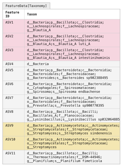
Figure 9:Assigning taxonomy to observed sequences. Your FeatureData[Sequence] artifact (Figure 5b) can be provided to a TaxonomicClassifier (Figure 8c) to generate taxonomic annotations in a FeatureData[Taxonomy] artifact. Each ASV sequence is run through the TaxonomicClassifier, and the most specific assignment that meets or exceeds the confidence threshold is assigned to the ASV. Some ASVs (e.g., ASV1 or ASV4) may only have acceptable assignment confidence at higher levels (genus and domain, respectively), while others (e.g., ASV2 and ASV3) may be assigned to the species level.
The ASV shading from Figure 7 is reintroduced here to illustrate that clustering into OTUs can mask true biological diversity present in the samples.
The classify-sklearn action assigns a confidence value between 0.0 and 1.0 (inclusive) to every taxonomic level it assigns to each input sequence.
The annotation that will be generated as output is then assigned to the most specific taxonomic label for which the confidence is above a user-defined threshold (default 0.70).
When reviewing Figure 9, you can see that some ASVs have higher resolution (i.e., “deeper” or “more specific”) assignments than others.
For example, ASV2 gets a species-level assignment, while ASV1 gets a genus-level assignment, and ASV4 only gets a domain-level assignment.
This means that ASV2’s species assignment was assigned with a confidence greater than or equal to 0.70, while ASV4 received a phylum-level assignment at a confidence less than 0.70.
Low resolution assignments can happen for a few reasons including: that a close representative to the sequence in question is not represented in the database, either because you’re working with an uncommon or previously unknown sequence or because you have a sequence that doesn’t represent one found in nature, for example as a result of PCR error; or that there is low information content in your amplicon for differentiating certain taxa (i.e., two species in the same genus have identical 16S sequences, so you can’t tell them apart from the sequencing data you have).
It’s normal to have some features, like ASV4 in Figure 9, that have low resolution taxonomy assignments.
If many of your sequences are in that category, it may indicate that there is a problem with your sequencing data.
To get an initial look at the taxonomic classifications, we can integrate taxonomy in the tabulate-seqs summary, like the one we generated above.
In this command, we are providing a label for the taxonomy.qza input, which will label the database source in the resulting visualization.
This is possible because this input is defined as a Collection, so we could provide multiple FeatureData[Taxonomy] artifacts as input to this step (for example, to compare taxonomy assignments obtained by different classifiers).
qiime feature-table tabulate-seqs \
  --i-data asv-seqs-ms2.qza \
  --i-taxonomy GTDB_r202_SpeciesReps:taxonomy.qza \
  --m-metadata-file asv-frequencies-ms2.qza \
  --o-visualization asv-seqs-ms2.qzv
asv_frequencies_md = asv_frequencies_ms2.view(Metadata)
taxonomy_collection_artifact_collection = ResultCollection({
'GTDB_r202_SpeciesReps': taxonomy,
})
asv_seqs_ms2_viz, = feature_table_actions.tabulate_seqs(
data=asv_seqs_ms2,
taxonomy=taxonomy_collection_artifact_collection,
metadata=asv_frequencies_md,
)asv_frequencies_md <- asv_frequencies_ms2$view(Metadata)
taxonomy_collection_artifact_collection = ResultCollection(dict(
'GTDB_r202_SpeciesReps' = taxonomy
))
action_results <- feature_table_actions$tabulate_seqs(
data=asv_seqs_ms2,
taxonomy=taxonomy_collection_artifact_collection,
metadata=asv_frequencies_md,
)
asv_seqs_ms2_viz <- action_results$visualizationasv_frequencies_ms2_as_md = use.view_as_metadata('asv_frequencies',
asv_frequencies_ms2)
taxonomy_collection = use.construct_artifact_collection(
'taxonomy_collection', {'GTDB_r202_SpeciesReps': taxonomy}
)
use.action(
use.UsageAction(plugin_id='feature_table',
action_id='tabulate_seqs'),
use.UsageInputs(data=asv_seqs_ms2,
taxonomy=taxonomy_collection,
metadata=asv_frequencies_ms2_as_md),
use.UsageOutputNames(visualization='asv_seqs_ms2'),
)Recall that our asv-seqs.qzv visualization allows you to easily BLAST the sequence associated with each feature against the NCBI nt database.
This visualization has the same functionality, but now includes the taxonomic annotation of the ASVs as determined using QIIME 2.
Using the asv-seqs-ms2.qzv Visualization created here, compare the taxonomic assignments with the taxonomy of the best BLAST hit for a few features.
Solution to Exercise 8
The highest frequency feature, c6c3ab4e828fb40d6e05967b7aac9338, is labeled as follows by our classifier:
d__Bacteria;p__Firmicutes_A;c__Clostridia;o__Lachnospirales;f__Lachnospiraceae;g__Blautia_AThis aligns well with our BLAST results when viewed collectively.
In the solution to Exercise 6, we noted that the best matches included hits in the Blautia genus, but no conclusive species label.
This is exactly what our classifier reports: notice that the assignment ends after g__Blautia_A, with no species level assignment.
The lack of a species-level assignment is a result of the classifier not being able to make a confident species-level assignment.
It’s worth noting that our consideration of this sequence in Exercise 6 as belonging to the Blautia genus required manual review of many top BLAST hits, as the first hit described it simply as an uncultured bacterium clone. Additionally, several of the top scoring BLAST assignments viewed individually could have led to over-confidence in a species assignment.
One additional note: when GTDB assigns a letter to a taxonomic label (like the A in Blautia_A here) that means that they have observed that the previously named group (Blautia, in this case) is not monophyletic based on the multi-gene trees that guide their taxonomy.
The A therefore indicates one monophyletic grouping of taxa in what are known as Blautia.
Taxonomic analysis
At this point, we have what we need to get our first high-level look at our samples.
Specifically, we can see which taxa are present in our samples.
This is generally viewed through a taxonomic barplot (Figure 10).
The QIIME 2 taxonomic barplots enable viewing the observed taxonomic composition of our samples by converting all feature frequencies to relative frequencies (Figure 10a), and then grouping features and summing their counts based on their taxonomic annotation (Figure 9).
Taxonomic barplots can then be presented for different taxonomic levels: in our schematic figures Figure 10b presents the phylum-level composition, and Figure 10c presents the genus level composition.
(Features without assignment at the current taxonomic level are grouped based on their deepest level of assignment: for example, in Figure 10b the d__Bacteria level groups all features that are assigned to d__Bacteria but not to a phylum.)
These plots allow us to observe a pattern in the schematic data: the sample composition transitions from more human-excrement-like in the early composting timepoints to more food-compost-like in the later timepoints.
We can also see which taxa may be responsible for this change in composition or may be responding to changing composting conditions over time.
(Refer to Figure 3 if you need to remind yourself of the sample types.)
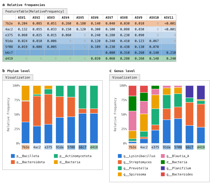
Figure 10:Taxonomic composition of samples as stacked bar plots. Taxonomic composition barplots are a common summary visualization of samples. These represent the feature table as relative abundances (panel a), with ASVs grouped based on their taxonomic labels (e.g., Figure 9). Taxonomic groupings can be presented at different focal levels, such as phylum (panel b) or genus (panel c). If an ASV doesn’t have an assignment at the focal level (e.g., ASV4 for the genus plot), it will generally be annotated at the lowest level it was assigned (hence d__Bacteria in the genus-level plot).
In the constructed data, we can see from this plot that some taxa (e.g., Blautia-A) decrease in abundance during the composting process, while others (e.g., Streptomyces) increase in abundance. The choice of taxonomic level changes what is visible: at phylum level the transition is less apparent, in part because Bacillota includes the gut-associated Blautia-A and the compost-associated Lysinibacillus and Planifilum.
Generate taxonomic barplots for the tutorial data with the following command and then open the Visualization.
qiime taxa barplot \
  --i-table asv-table-ms2.qza \
  --i-taxonomy taxonomy.qza \
  --m-metadata-file sample-metadata.tsv \
  --o-visualization taxa-bar-plots.qzv
import rachis.plugins.taxa.actions as taxa_actions
taxa_bar_plots_viz, = taxa_actions.barplot(
table=asv_table_ms2,
taxonomy=taxonomy,
metadata=sample_metadata_md,
)taxa_actions <- import("rachis.plugins.taxa.actions")
action_results <- taxa_actions$barplot(
table=asv_table_ms2,
taxonomy=taxonomy,
metadata=sample_metadata_md,
)
taxa_bar_plots_viz <- action_results$visualizationuse.action(
use.UsageAction(plugin_id='taxa',
action_id='barplot'),
use.UsageInputs(table=asv_table_ms2,
taxonomy=taxonomy,
metadata=sample_metadata),
use.UsageOutputNames(visualization='taxa_bar_plots'))Solution to Exercise 9
The most dominant phylum in the Human Excrement samples appears to be p__Firmicutes_A followed by p__Bacteroidota.
In the Human Excrement Compost samples, the dominant phylum appears to be p__Proteobacteria, followed by p__Bacteroidota.
p__Bacteroidota abundance appears to be positively correlated with time, and p__Actinobacteriota may be negatively correlated with time, but these patterns are not perfect and somewhat hard to discern from this plot.
While taxa barplots can help us explore our data at a high level, such as comparing dominant phyla across sample types, in practice they are limited in their ability to help us understand more nuanced differences between our samples. And, as our data increases in size, these plots become increasingly hard to interpret. For example, try comparing the genus-level composition of adjacent timepoints: for a few different values of x, can you tell if timepoint x is more similar to timepoint x-1 or x+1 at the genus level? For this type of question, we need more quantitative approaches, and this is where alpha and beta diversity metrics help us. Generating a taxonomy barplot is almost always an early step in an analysis, and something that is referred back to when considering other results. It is also useful for assessing whether your sample compositions align with your expectations, so can be used as a sanity check of the data. It rarely, if ever, represents a key finding on its own.
Even sampling
One additional topic must be considered before we move on to alpha and beta diversity metrics, and that is the variation in the number of sequences obtained per sample (the sequencing depth) that is observed across samples in modern DNA sequencing runs.
Refer to Figure 11a, which presents our feature table alongside the sequencing depth (labeled Total frequency) for each sample following quality control (Figure 11b).
Notice that the sequencing depth for sample 4ac2 is approximately 20 times that of sample 5f08.
Differences in the sequencing depth across samples in an amplicon-based microbiome study generally are thought to be stochastic, rather than representative of true differences across samples (with an exception being very low microbial biomass samples, which can have very low sequencing depth because there are few microbial cells to sequence).
This difference can however impact the diversity metrics that we calculate on those samples, such that they may appear to be different as a result of the sampling depth obtained in each, rather than as a result of true biological differences between the samples.

Figure 11:Rarefying feature tables to achieve an even sampling depth across all samples. Samples from a single sequencing run often differ in sequencing depth (panels a and b). In general, this doesn’t represent the biology of the samples but rather is an artifact of the sequencing. Many of the diversity metrics that are applied to feature tables are sensitive to differences in sequencing depth, so this must be normalized. Rarefying a feature table is the most common way of achieving this normalization, and involves selecting an even sampling depth and then subsampling counts at random from all samples up to that depth without replacement. Samples with sequencing depth less than the even sampling depth are excluded from the resulting rarefied feature table. Panels c and d illustrate even sampling to 1800 sequences per sample. Because sample 5f08 had only 640 sequences, it is excluded from the rarefied table in panel c. Panels e and f illustrate even sampling to 8000 sequences per sample. All samples with fewer than 8000 sequences are excluded from the rarefied table in panel e.
As you can see, selecting an even sampling depth forces you to decide between excluding samples and excluding sequences. It is generally considered a “necessary evil”. Subsampling one time, as illustrated here, is rarefying. The more robust approach, rarefaction, rarefies multiple times and averages the resulting metrics.
The diversity calculations that follow will work from the depth-1800 table in panel c.
An analogy can be helpful here. Imagine a plant biologist (and not a very good one, for the sake of this example) who is interested in comparing the number of plant species found in the Sonoran Desert to that observed in the Costa Rican rainforest. To do this, they first survey 60 m² of the desert. Then, maybe because it’s harder to move around, they sample only 3 m² of the rainforest. When they get back to the lab, they tally up their results and conclude that there are more species of plant in the desert than there are in the rainforest. (Remember—they are not a very good biologist!) While this observation sounds quite surprising, we know there is a methodological flaw: they expended more effort counting species in the desert, so it’s not surprising that they found more species.
The land area sampled is an analog for the number of sequences collected in our microbiome study: if we obtain more sequences for some samples, we’re effectively expending more effort sampling them, and it shouldn’t be surprising if that impacts findings such as the count of the number of ASVs observed in each sample. Differences in sampling depth also impact more complex metrics of sample diversity.
This is generally addressed in microbiome studies by selecting a sequencing depth to normalize all samples for diversity metric computation.
This is referred to as the even sampling depth and selecting this is a common source of questions; we’ll provide guidance on this next.
Figure 11c-d illustrates selecting an even sampling depth of 1800 for the example feature table.
When this is done, the sequence counts are resampled for each sample (typically without replacement) until the total count for that sample is 1800.
This is repeated for all samples, and if a sample has fewer than 1800 sequences, that sample will be dropped from the resulting table.
This is the case for sample 5f08 in Figure 11c: it is the sample with the lowest sampling depth in this feature table.
At an even sampling depth of 1800, it would be excluded from diversity metric calculations.
Performing a single resampling of the feature table to a specific even sampling depth (e.g., as illustrated in either Figure 11c or Figure 11e) is referred to as rarefying the feature table. The resulting diversity metrics however are sensitive to the specific sampling that was performed, and as is clear by comparing the “Total” rows in Figure 11d and Figure 11f to that in Figure 11b, it results in excluding a lot of the data that was collected during sequencing. The approach that we’ll use here, rarefaction, performs the resampling step n times, and then averages downstream results. This results in more robust diversity metric calculations, and ensures that those diversity metrics have accounted for more of the underlying data. We’ll apply that approach here using the q2-boots plugin, after illustrating the simpler case of computing diversity metrics from the rarefied feature table in Figure 11c.
If our plant biologist wanted to normalize their sampling effort by these approaches, they could consider a few options assuming they recorded the specific location(s) where each species was observed during their sampling. They could apply an approach like rarefying by selecting at random a 3 m² subplot from the desert, and tallying the desert plant species count in that subplot for comparison to the rainforest plant count. Or, more robustly, they could randomly sample multiple 1 m² subplots from both the desert and rainforest, tally the average number of plant species in each subplot, and compare those averages. (Even in this case however, our plant biologist is to be pitied: without multiple replicates per site, any results they come up with are not likely to be very convincing.)
Selecting an even sampling depth
Selecting an even sampling depth is a balance between discarding sequences and discarding samples. If a lower even sampling depth is chosen to avoid excluding samples, each sample is represented by fewer sequences. If a higher depth is chosen to represent each sample by more sequences (see Figure 11e-f), then more samples may be discarded.
Generally, selecting an even sampling depth requires a few important considerations.
First, you want it to exclude samples where the sequencing seems to have failed—this might be those where the sampling depth is in the ones, tens, or hundreds.
It’s not a bad idea to remove these from your feature table entirely, using qiime feature-table filter-samples.
Then, you want to set it low enough that you’re losing an acceptable number of samples, which is a painful decision to make but is a choice that needs to be made on a per-study basis.
The asv-table-ms2.qzv that you created for Exercise 7 can help you explore the trade-off between number of sequences and number of samples discarded.
Experiment with the dropdown box and the slider bar in the Interactive Sample Detail tab.
Selecting the SampleType metadata category will group your samples by their type allowing you to see how many samples you’ll lose from each category for a given sampling depth.
Think about which categories are the ones that you need to compare, and ensure that you’re selecting an even sampling depth that retains a sufficient number of samples in each of those categories.
Finally, you ideally want to choose an even sampling depth where you expect your diversity metrics to begin to stabilize, which is something you can assess with alpha and beta rarefaction analyses.
Figure 12a illustrates a simplified alpha rarefaction plot. In an alpha rarefaction analysis, you step through a series of even sampling depths and generate n feature tables at each step. You then compute an alpha diversity metric (observed features, in Figure 12a), and you observe where those values begin to plateau for each of your samples or sample categories. That gives you an idea of where you expect your alpha diversity values to stabilize, and in general selecting a value in that range that retains as many samples as possible is ideal. Notice that the observed features values have stabilized in Figure 12 at the two example even sampling depths that we explored in Figure 11, but an even sampling depth of 1800 retains six samples while an even sampling depth of 8000 retains only three samples. (Because the constructed data used in the figures is so simplistic, our alpha diversity values stabilize very quickly and indicate that a lower depth could be selected for this data to retain all seven samples. For the sake of illustration though, we’ll select the value of 1800 so that our downstream results represent the more common scenario where some samples that were sequenced must be excluded from diversity analysis.)
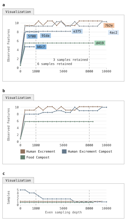
Figure 12:Alpha rarefaction plot of observed features as a function of even sampling depth. For an alpha rarefaction plot (panel a), the feature table is subsampled without replacement at evenly spaced depths and a specific alpha diversity metric is computed on each of those tables. In this plot, there are 20 even sampling depths ranging from 1 to 10,000, and the observed features metric is calculated on each feature table. This allows you to assess several aspects of the data, including relative alpha diversity of the samples, the even sampling depth at which each sample appears to have been “fully sampled” (meaning that additional sequences do not yield additional alpha diversity), and the sampling depth at which specific samples are dropped. The dashed vertical lines mark 1800 and 8000, the two candidate even sampling depths explored in Figure 11, each labelled with the number of samples that would be retained if that sampling depth was selected. QIIME 2’s alpha-rarefaction command repeats each even sampling depth 10 times and plots the median value for each (sample, even sampling depth) pair. Panels b and c mirror those generated by QIIME 2’s alpha-rarefaction command, where samples are generally grouped into single lines by metadata. In panel b, our HEC samples are all grouped together, and in this view it is not immediately clear how many samples are retained at each even sampling depth. Panel c illustrates this information.
Figure 12b-c mirror the plots generated by QIIME 2’s alpha-rarefaction action, which we will run next.
In the QIIME 2 alpha rarefaction plots, samples are often grouped by metadata (e.g., all HEC samples are grouped into one line in Figure 12b), to help with visualizing these plots for large collections of samples.
The secondary plot (illustrated in Figure 12c) presents how many samples are retained for each group at each even sampling depth.
We can generate an alpha rarefaction plot for the tutorial data using the alpha-rarefaction action.
This visualizer computes one or more alpha diversity metrics at multiple sampling depths, in steps between 1 (optionally controlled with min-depth) and the value provided as max-depth.
At each sampling depth step, 10 rarefied tables will be generated, and the diversity metrics will be computed for all samples in the tables.
The number of iterations (rarefied tables computed at each sampling depth) can be controlled with the iterations parameter.
The diversity values will be plotted for each sample at each even sampling depth, and samples can be grouped based on metadata in the resulting visualization if sample metadata is provided.
The value that you provide for max-depth should be determined by reviewing the “Frequency per sample” information presented in the asv-table-ms2.qzv file.
In general, choosing a value that is somewhere around the median frequency seems to work well, but you may want to increase that value if the lines in the resulting rarefaction plot don’t appear to be leveling out, or decrease that value if you seem to be losing many of your samples due to low total frequencies closer to the minimum sampling depth than the maximum sampling depth.
qiime diversity alpha-rarefaction \
  --i-table asv-table-ms2.qza \
  --p-max-depth 260 \
  --m-metadata-file sample-metadata.tsv \
  --o-visualization alpha-rarefaction.qzv
import rachis.plugins.diversity.actions as diversity_actions
alpha_rarefaction_viz, = diversity_actions.alpha_rarefaction(
table=asv_table_ms2,
max_depth=260,
metadata=sample_metadata_md,
)diversity_actions <- import("rachis.plugins.diversity.actions")
action_results <- diversity_actions$alpha_rarefaction(
table=asv_table_ms2,
max_depth=260L,
metadata=sample_metadata_md,
)
alpha_rarefaction_viz <- action_results$visualizationuse.action(
use.UsageAction(plugin_id='diversity',
action_id='alpha_rarefaction'),
use.UsageInputs(table=asv_table_ms2,
max_depth=260,
metadata=sample_metadata),
use.UsageOutputNames(visualization='alpha_rarefaction'))The Visualization will have two plots. The top plot is an alpha rarefaction plot, and is primarily used to determine if the richness of the samples has been fully observed or sequenced. If the lines in the plot appear to “level out” (i.e., approach a slope of zero) at some sampling depth along the x-axis, that suggests that collecting additional sequences beyond that sampling depth would be unlikely to result in the observation of additional features. If the lines in the plot don’t level out, this may be because the richness of the samples hasn’t been fully observed yet (because too few sequences were collected), or it could be an indicator that a lot of sequencing error remains in the data (which is being mistaken for novel diversity).
The bottom plot in this Visualization is important when grouping samples by metadata. It illustrates the number of samples that remain in each group when the feature table is rarefied to each sampling depth. If a given sampling depth d is larger than the sequencing depth of a sample s (i.e., the number of sequences that were obtained for sample s), it is not possible to compute the diversity metric for sample s at sampling depth d. If many of the samples in a group have lower total frequencies than d, the average diversity presented for that group at d in the top plot will be unreliable because it will have been computed on relatively few samples. When grouping samples by metadata, it is therefore essential to look at the bottom plot to ensure that the data presented in the top plot is reliable.
Solution to Exercise 10
The Microbe Mix sample appears to level out quickly. The Human Excrement, Human Excrement Compost, and Food Compost additionally appear to level out, though there appears to be some positive slope remaining. Other sample types appear unstable, but by comparing with the plot underneath the rarefaction plot we can see that those groups are based on relatively few samples at the higher sequencing depths.
There are many QIIME 2 Forum posts on the topic of selecting an even sampling depth, and some video content on the QIIME 2 YouTube channel. You can refer to those, and discuss with others on the forum if you have questions when making this decision for your analysis. We recommend keeping in mind a couple of points when deciding on a sampling depth. First, relative diversity metrics tend to be quite stable down to low even sampling depths. For example, if you see a pattern of similarity between your samples at a relatively high even sampling depth, that pattern tends to also be present at relatively lower even sampling depths within reason. It never hurts to experiment with multiple even sampling depths and compare the results to assess whether your conclusions change. You can even present the results from different even sampling depths as supplementary analysis in a research paper—for example, by focusing on a lower even sampling depth that retains more samples in your main text figures, but then presenting results obtained with higher even sampling depths in a supplement to confirm that the patterns you presented are still apparent. Second, if you’re using the rarefaction approach in q2-boots, which we illustrate in this tutorial, you can feel confident knowing that even if you choose a lower even sampling depth that discards a large fraction of your sequences, because the rarefy step will be run multiple times, those sequences will be used to define representative sample composition. In other words, even though an individual rarefy step may consider only a small fraction of your sequences, the multiple iterations (default of 100) will consider a much larger fraction.
Alpha and beta diversity analysis background
Background: alpha and beta diversity metrics (Figure 13 - Figure 18)
Alpha (α) and beta (β) diversity analysis are common next steps in a microbiome amplicon analysis, and facilitate interpretation of the relative similarities and differences across samples. α diversity metrics are computed from a single sample at a time, and as a result are often referred to as “within-sample” diversity. β diversity metrics on the other hand are computed on pairs of samples, and are therefore often referred to as “between-sample” diversity.
Experimental choices ranging from DNA extraction protocol through PCR primer choice and bioinformatics processing, and experimental artifacts such as sequencing depth, all impact our observation of microbiome sample composition, and α and β diversity should therefore always be considered a function of those parameters in addition to our observed sample composition. For this reason, care must always be taken if trying to compare microbiome compositions across studies.
There are many diversity metrics implemented in QIIME 2—about 30 α metrics and 25 β diversity metrics. Each tells us about a different aspect of the data, and computing and comparing multiple diversity metrics can help you understand different features of your data. For example, stepping back from biology for a moment, imagine that you want to compute the physical distance between two cities. There are various ways that you could measure this, and the way you choose to measure it depends on what you need to do with that distance. You could draw a straight line between the two cities on a map, measure that line, and you’d have a distance between the cities. But, if you’re driving between the cities, that distance won’t be very relevant unless there is a road that connects the cities by the line that you’ve drawn. In this case, a more relevant distance will be that of the shortest drivable route between the two cities, achieved by measuring the lengths of the roads composing the route. Just as there are many ways to compute the distance between two cities, there are many ways to assess the diversity of biological communities.
In this section, we’re going to briefly cover three independent categorizations of diversity metrics and then mention specific examples of these that can be computed in QIIME 2. Detailed discussion of each metric is beyond the scope of this tutorial document, but there is plenty of online content about these.
α Diversity versus β Diversity
The first category of diversity metrics we’ll discuss is α diversity versus β diversity. As described above, α diversity is computed on a single sample. These methods generally encompass measures of richness and/or evenness of a sample. The simplest of these is observed features, which we discussed above in the context of Figure 12. This is a simple count of the features observed in a sample with a frequency of greater than zero. Figure 13a presents this for each sample based on the evenly sampled feature table in Figure 11c. To ensure that you understand it, as well as the other diversity metrics that are presented in this section, you can compute them by hand on the Figure 11c feature table and confirm that you obtain the same results that you see here. The result of computing an α diversity metric on a set of samples is a vector of alpha diversity values.
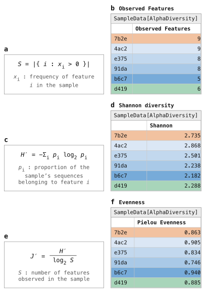
Figure 13:Three identity-based alpha diversity metrics. Three alpha diversity metrics, Observed Features (panels a and b), Shannon Diversity (panels c and d), and Pielou’s Evenness (panels e and f) are applied to the feature table in Figure 11c. Each results in a SampleData[AlphaDiversity] artifact, which summarizes each sample in a single value. Logarithms in these formulas are base 2, matching QIIME 2.
β diversity is computed on pairs of samples, and most commonly represents a distance between samples. A lower β diversity value between a pair of samples suggests that they are more similar; a higher β diversity value suggests that they are more dissimilar. A simple β diversity metric is Jaccard dissimilarity, which is illustrated in Figure 14a-b. The Jaccard dissimilarity between samples A and B is computed as one minus the number of features present in both samples A and B divided by the number of features present in either sample A or B. Again, you can work through the formula presented in Figure 14a on the feature table in Figure 11c, and check your answers against Figure 14b to confirm that you understand how this metric is computed. The result of computing a β diversity metric on a set of samples is a distance matrix, where each cell stores the distance between a corresponding pair of samples. True measures of distances between samples (a category that most but not all β diversity metrics fall into) result in distance matrices that guarantee four specific criteria:
The distance matrix is hollow (or has zeros on the diagonal), indicating that the distance between a sample and itself will always be zero.
The distance matrix is symmetric, indicating that the distance between sample A and B will always be equal to the distance between sample B and A.
Distances between samples will always be greater than or equal to zero.
Distances adhere to the triangle inequality, such that the distance between samples A and C will always be less than or equal to the distance between sample A and B plus the distance between B and C.
Some operations that are applied to distance matrices downstream assume these characteristics, so it’s worth being aware of these criteria.

Figure 14:Two identity-based beta diversity metrics. Two beta diversity metrics, Jaccard distance (panels a and b) and Bray-Curtis distance (panels c and d), are applied to the feature table in Figure 11c. Each results in a DistanceMatrix object, where the values are interpreted as the dissimilarity between the pair of samples it represents (larger values indicate less similar samples).
Qualitative versus quantitative
The next category we’ll discuss here is qualitative versus quantitative diversity metrics. Qualitative diversity metrics consider only the presence or absence of features in the feature table, not their actual counts. Quantitative diversity metrics, on the other hand, consider the counts of the features. The two metrics we discussed in the previous section, observed features and Jaccard dissimilarity, are both qualitative diversity metrics: notice that each only considers which features are and are not observed on a per-sample basis. Figure 13c-f and Figure 14c-d present quantitative α and β diversity metrics, respectively. While it might seem that qualitative diversity metrics add little, remember that the extraction, PCR, and sequencing steps in generating our data can all obscure the true abundances of features (e.g., because of preferential extraction of some taxon’s DNA over another). It is common to compute both qualitative and quantitative metrics and present the two side-by-side, and to remember that neither is a perfect representation of the biology of our samples.
Identity-based vs. relatedness-based
The final category we’ll cover here is identity-based diversity metrics versus relatedness-based diversity metrics. An identity-based diversity metric treats all features as independent, ignoring any possible relationship between them. These metrics are identity-based in the sense that a feature’s identity is the only information they use: two observations either represent the same feature or different features, and all different features are treated as equally distinct, whether their sequences differ by one nucleotide or many. Relatedness-based metrics, on the other hand, incorporate relationships between features. The metrics represented in Figure 13 and Figure 14 are all identity-based metrics.
The most widely used approach for incorporating feature relatedness in diversity metric computation in microbiome studies is through phylogenetic inference: in addition to the feature table, a phylogenetic tree where the feature ids are the tips in the tree (Figure 15) is included as input to the diversity metric, and the distance between the tips in the tree is interpreted as the relatedness of features by the diversity metric. QIIME 2 supports several phylogenetic diversity metrics, including Faith’s Phylogenetic Diversity (Figure 16), unweighted UniFrac (Figure 17b-c), and weighted UniFrac (Figure 17d-e).
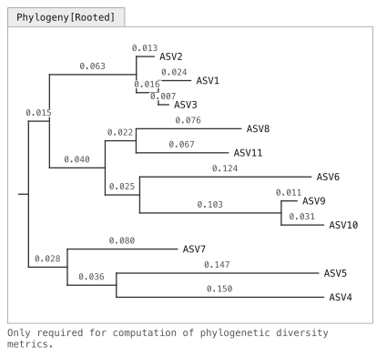
Figure 15:A rooted phylogeny of the ASV sequences. A rooted phylogenetic tree relating the eleven ASV sequences. Horizontal distances are drawn to scale and every branch is labelled with its length in substitutions per site; vertical placement carries no information. Relatedness-based diversity metrics can use a phylogenetic tree to represent the relatedness between features.
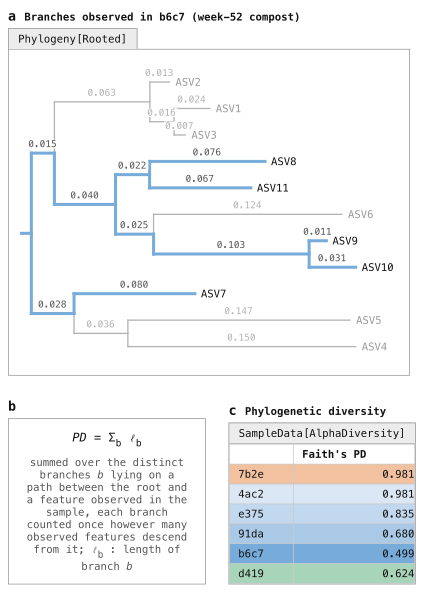
Figure 16:Alpha diversity with Faith’s Phylogenetic Diversity. Instead of counting a sample’s features, Faith’s phylogenetic diversity (PD) sums the lengths of the branches that are represented in a sample. This is done by identifying which ASVs (tips in the tree) are observed in a sample, tracing each of those to the root of the tree (panel a), and then summing those “observed branch lengths” (panel b). Those values are represented in a SampleData[AlphaDiversity] artifact (panel c), like the identity-based metrics presented in Figure 13.

Figure 17:Beta diversity with UniFrac. UniFrac is an approach for integrating relatedness in beta diversity metrics. Like Faith’s PD, it leverages branch lengths, but this time focusing on each pair of samples in the data set. Panel a illustrates this for samples e375 (blue) and d419 (green). The branch length that is present in only one of the two samples (where there is only a single colored trace in panel a, such as the branches leading to ASVs 1–3 and ASV10) is referred to as the unique branch length. The branch length that is present in either of the two samples (where there are one or two colored traces in panel a) is referred to as the observed branch length. The unique branch length is divided by the observed branch length, yielding the unique fraction of the observed branch length for the pair of samples (from which UniFrac derives its name). Unweighted UniFrac (panels b and c) considers only presence/absence of features, while Weighted UniFrac (panels d and e) weights branches based on feature abundances.
Relatedness can alternatively be integrated in other ways, such as through shared kmer composition as in the q2-kmerizer Bokulich, 2025 plugin. Briefly, this works by decomposing each ASV sequence into its constituent length-k words, or kmers, as illustrated in Figure 18a. The feature table is then updated such that the features become these kmers, and their per-sample counts are the sum of the counts of the ASV(s) in which each was observed (Figure 18b). This encodes feature relatedness directly in the feature table: evolutionarily closer sequences share more kmers, so diversity metrics computed on it integrate that relatedness. A point worth remembering is that, as currently implemented in QIIME 2, identity-based metrics are applied to this kmer feature table, so feature relatedness is integrated through the table, not the metrics themselves.

Figure 18:Kmerization of ASV sequences and a feature table. An alternative approach for relatedness-based diversity metrics splits sequences into their constituent kmers (panel a), and then expands the feature table from ASVs to kmers (panel b). The count of a kmer in a sample is the summed count of every ASV whose sequence contains it. More closely related ASVs share more kmers with each other, and as a result computing identity-based diversity metrics on this kmer table results in diversity values that implicitly integrate feature relatedness.
These approaches achieve the same goal of integrating feature relatedness, but in different ways: phylogenetic relationships are inferred from the data using a series of models (for multiple sequence alignment, phylogenetic reconstruction, and tree rooting), while kmer-based relatedness is a directly measured property of the observed data. The kmer approach is objectively simpler: it’s a deterministic alignment-free approach with a single free parameter, k, that provides only rough estimates of feature relatedness. Phylogenetic inference involves many parameters and yields an explicit hypothesis about the evolutionary relationships between the features. The phylogenetic tree, when correct, has considerably more value (branch lengths, evolutionary placement of novel organisms), but each step carries assumptions and errors can propagate forward into the diversity metric. In practice, the simpler kmer-based diversity calculations appear to perform no worse than phylogeny-based methods Bokulich, 2025.
Relatedness-based diversity metrics and identity-based diversity metrics provide different perspectives for resolving differences between microbiome samples, and both are common in practice.
Phylogenetic inference
QIIME 2 offers a few ways to build phylogenetic trees for use in computing phylogenetic diversity metrics, including a reference-based approach in the q2-fragment-insertion plugin Janssen et al., 2018 and de novo (i.e., reference-free) approaches in the q2-phylogeny plugin. Each of these methods has benefits and drawbacks. The reference-based approach, by default, is specific to 16S rRNA marker gene analysis. This uses a pre-computed reference tree and then inserts the observed sequences into that tree. De novo tree building, an alternative, doesn’t rely on any outside information so can be used with any phylogenetically informative marker gene (not just 16S). Reference-based tree building is generally considered to result in a higher-quality tree than de novo tree building, but you need to have a tree that you trust to begin with. Reference-based tree building is illustrated in the Parkinson’s Mouse tutorial, and de novo tree building is illustrated in the Moving Pictures tutorial. In the gut-to-soil tutorial, we opt for the simpler kmer-based approach for computing relatedness-based diversity metrics so we will skip the phylogenetic reconstruction step.
Running the kmer-diversity Pipeline
In the past few sections we’ve covered a lot of background while running very few commands.
We’re going to pull this together in this section by running rarefaction (i.e., multiple iterations of rarefying) and using the resulting evenly sampled feature tables to compute qualitative and quantitative relatedness-based α and β diversity metrics.
This is a complex but very common workflow, so QIIME 2 provides a single Pipeline, kmer-diversity, to do all of this work in a single step in the q2-boots Raspet et al., 2025 plugin.
The q2-boots plugin also provides all the constituent actions, so you can run the steps that are described here separately, but in practice that is not common.
While kmer-diversity is accessed through q2-boots, the Pipeline leverages other QIIME 2 plugins including q2-kmerizer Bokulich, 2025, q2-vizard, and q2-diversity.
You can learn more about the rarefaction-based workflows in q2-boots and the kmer-based diversity analysis methods in q2-kmerizer in the respective papers about those plugins Raspet et al., 2025Bokulich, 2025.
The following list describes the steps of the kmer-diversity Pipeline, with specific parameters that the user can set presented in monospace font (e.g., sampling-depth).
Resample the input feature table (Figure 5a) to contain exactly
sampling-depthsequences per sample, either by bootstrapping or rarefaction,ntimes. Samples with fewer thansampling-depthsequences will be removed from the feature table and not included in the subsequent steps, as illustrated in Figure 11c and Figure 11f. This will result innfeature tables (Figure 19a).For each feature table resulting from step 1, using the input sequences (Figure 5b), kmerize all sequences (e.g., Figure 18a) into kmers of length
kmer-size.[2] Use this information to create one kmer table per resampled feature table (e.g., Figure 18b). This will result innkmer-based feature tables.Compute
alpha-metricsandbeta-metricson each of the kmer tables resulting from step 2.[3] This will result inndiversity metric computations per diversity metric (Figure 19b and Figure 19d). The metrics computed by default are:Alpha diversity
Beta diversity
For each diversity metric, average its
nresults (Figure 19c and Figure 19e). These results can be used in subsequent analysis steps (e.g., ordination, statistical modeling, machine learning).Perform PCoA ordination on the averaged beta diversity distance matrices resulting from Step 4.[4]
Generate an interactive q2-vizard scatter plot that contains all user-provided sample metadata, all averaged alpha diversity metrics, and the first three ordination axes for all PCoA matrices computed in step 5 (e.g., Figure 20).
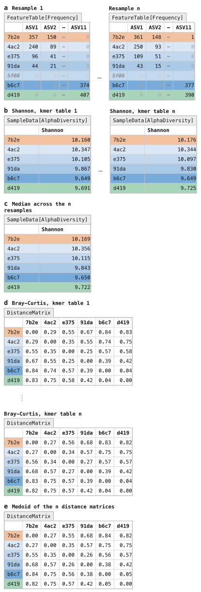
Figure 19:kmer-diversity workflow in q2-boots. The kmer-diversity Pipeline integrates the kmer diversity approach with repeated rarefying for rarefaction- and relatedness-based diversity metric computation. Each ASV table is sampled to an even sampling depth (Figure 11) n times (panel a). Each of the n rarefied ASV tables is then kmerized (Figure 18), and identity-based alpha diversity (Figure 13) and beta-diversity (Figure 14) metrics are computed on each kmer table. This results in n SampleData[AlphaDiversity] Artifacts per alpha diversity metric (panel b) which are subsequently averaged to generate the final output (panel c), and n DistanceMatrix Artifacts per beta diversity metric (panel d) which are subsequently averaged to generate the final output (panel e). The Pipeline yields one SampleData[AlphaDiversity] Artifact (panel c) and one DistanceMatrix Artifact (panel e) per diversity metric as output. Those averaged artifacts can be used in any downstream work that operates on SampleData[AlphaDiversity] or DistanceMatrix artifacts.
There are three required parameters that the user must set to define this run.
The most difficult to determine is the value to provide for the sampling-depth parameter.
Refer back to Selecting an even sampling depth above for discussion of this topic.
The user must also provide a value for n, the number of iterations of even sampling to run.
You should expect runtime to increase linearly with the setting of this parameter (such that n=1000 should take 100 times longer to run than n=10).
We recommend n=100 as a good starting point.
Finally, the user must additionally indicate whether each individual resampling step should occur with or without replacement, through the replacement parameter.
Sampling without replacement is rarefaction, and is most widely used.
Sampling with replacement is bootstrapping (the origin of the name q2-boots).
These produce nearly identical results Raspet et al., 2025 and we recommend the field does additional work to determine if one or the other of these methods is better in practice.
As of this writing (on 2 October 2026), we recommend sampling without replacement to align with the most commonly used approach.
Solution to Exercise 11
Importantly, remember that the even sampling depths we’re viewing here are extremely low because this is a small subset of a single sequencing run. At an even sampling depth of 96, we would retain 74 samples (75%) and 7,104 (24%) of our sequences. At 140 sequences per sample, we would retain 62 samples (63%) and 8,680 (29%) of our sequences. At 180 sequences per sample, we would retain 55 samples (56%) and 9,900 (33%) of our sequences. Our alpha rarefaction curve suggests that a higher value (in the 180 range) would be more appropriate because the richness begins to stabilize. This is likely the most reasonable value to choose, but in this dataset it unfortunately would result in losing nearly 50% of our samples. For the purpose of the tutorial, we’ll select 96 to retain 75% of our samples. Because we’re going to use rarefaction-based diversity calculations here, we can be less concerned about a lower number of sequences per sample.
Let’s now run kmer-diversity on the tutorial data, which will involve setting the three required parameters mentioned above.
Remember that we’re working with a small subset of a full sequencing run in this tutorial, to keep the runtime short for the tutorial.
As a result, the value used for sampling-depth here is very low.
Often, this might be closer to 10,000 for an Illumina run (as of 2026), but this is highly dependent on the sequencing run, the number of samples included, and other factors.
Additionally, to keep the runtime short, we set n to 10, and to align with the recommendation made earlier, we’ll generate the evenly sampled feature tables without replacement.
qiime boots kmer-diversity \
  --i-table asv-table-ms2.qza \
  --i-sequences asv-seqs-ms2.qza \
  --m-metadata-file sample-metadata.tsv \
  --p-sampling-depth 96 \
  --p-n 10 \
  --p-no-replacement \
  --output-dir boots-kmer-diversity
import rachis.plugins.boots.actions as boots_actions
action_results = boots_actions.kmer_diversity(
table=asv_table_ms2,
sequences=asv_seqs_ms2,
metadata=sample_metadata_md,
sampling_depth=96,
n=10,
replacement=False,
)
resampled_tables_artifact_collection = action_results.resampled_tables
kmer_tables_artifact_collection = action_results.kmer_tables
alpha_diversities_artifact_collection = action_results.alpha_diversities
distance_matrices_artifact_collection = action_results.distance_matrices
pcoas_artifact_collection = action_results.pcoas
kmer_diversity_scatter_plot_viz = action_results.scatter_plotboots_actions <- import("rachis.plugins.boots.actions")
action_results <- boots_actions$kmer_diversity(
table=asv_table_ms2,
sequences=asv_seqs_ms2,
metadata=sample_metadata_md,
sampling_depth=96L,
n=10L,
replacement=FALSE,
)
resampled_tables_artifact_collection <- action_results$resampled_tables
kmer_tables_artifact_collection <- action_results$kmer_tables
alpha_diversities_artifact_collection <- action_results$alpha_diversities
distance_matrices_artifact_collection <- action_results$distance_matrices
pcoas_artifact_collection <- action_results$pcoas
kmer_diversity_scatter_plot_viz <- action_results$scatter_plotuse.action(
use.UsageAction(plugin_id='boots',
action_id='kmer_diversity'),
use.UsageInputs(table=asv_table_ms2,
sequences=asv_seqs_ms2,
metadata=sample_metadata,
sampling_depth=96,
n=10,
replacement=False),
use.UsageOutputNames(
resampled_tables='resampled_tables',
kmer_tables='kmer_tables',
alpha_diversities='alpha_diversities',
distance_matrices='distance_matrices',
pcoas='pcoas',
scatter_plot='kmer_diversity_scatter_plot')
)boots-kmer-diversity/resampled_tables.zip| downloadboots-kmer-diversity/kmer_tables.zip| downloadboots-kmer-diversity/alpha_diversities.zip| downloadboots-kmer-diversity/distance_matrices.zip| downloadboots-kmer-diversity/pcoas.zip| downloadboots-kmer-diversity/scatter_plot.qzv| download | view
After computing diversity metrics, we can begin to explore the microbial composition of the samples in the context of the sample metadata. As you’re interpreting the results, remember that q2-kmerizer decomposes each sequence into its constituent kmers. This should be carefully considered when interpreting alpha diversity in particular, as the number of observed features (for example) would correspond to the number of unique kmers observed in a sample (representing the genetic diversity), not the number of unique sequences or taxa. For more information, read the q2-kmerizer paper Bokulich, 2025.
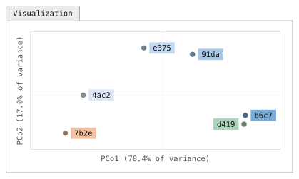
Figure 20:Ordination of the averaged kmer Bray-Curtis distances. Principal Coordinates Analysis (PCoA) scatter plots are a common way to visualize microbiome beta diversity. PCoA embeds the samples so that distances in the scatter plot approximate the distances in the DistanceMatrix, and the axes present how much of the total variance each coordinate explains. Each point represents a single sample, and coloring of points based on metadata is commonly used to aid in discovery of patterns. This plot suggests that through the composting process, the samples look less like fecal material and more like food compost in their microbial composition. The orientation of a PCoA axis is arbitrary. Here, axis 1 is drawn with human excrement at the left so the composting series reads left to right. The percentage on each axis is the share of the total variation in the distance matrix that the axis captures. That value is high here because this constructed data set has only six samples and was designed to model a simple transition along the composting time series; in real data with many samples and sources of variation a low percentage is normal. For example, the percent variation explained by Unweighted UniFrac PCoA axis 1 for Meilander et al. (2024) was 11.26% (the interactive Emperor plot is linked from Caporaso & Meilander (2025)).
Solution to Exercise 12
The samples appear to exhibit some clustering by SampleType.
If you want a more targeted view of any trends you see in your data, you can use the lineplot visualizer.
This provides a slightly less exploratory view of your data, with a fixed value on the x axis.
You can still cycle through all available numeric metadata columns on the y axis, utilize grouped coloring for all categorical metadata columns, and view the mean or median values for grouped data (if you have replicates in the metadata column you’re plotting on the x axis).
Solution to Exercise 13
On Axis 1, the HEC samples cluster closely with the Food Compost samples. These separate from each other on Axis 2. Because Axis 1 explains more variation than Axis 2, and because there is some overlap of the HEC and Food Compost samples on Axis 2, this suggests that the HEC is more similar to the Food Compost samples than the HE samples. Whew!
The Microbe Mix sample is most similar to one of the Food Compost samples. The Inside Toilet Pre Use samples also seem to cluster among the Food Compost samples, though one does appear to cluster clearly with the HE samples. The Bulking Material samples cluster between the HEC and Food Compost samples.
Bray-Curtis Axis 2 and Jaccard Axis 2 appear to be strongly correlated with observed features (and with each other). (Because the direction of axes is arbitrary in PCoA, differences in positive and negative correlation are not interesting.) Bray-Curtis Axis 1 and Jaccard Axis 1 appear to be strongly correlated with each other. For the HEC samples, there may be a weak negative correlation between Composting Time Point and observed features.
The Microbe Mix has the lowest microbial richness. This is easily observed by plotting observed features versus itself in this scatter plot.
Differential abundance testing with ANCOM-BC2
The final analysis step that we’ll cover here is identifying individual features that are differentially abundant across sample types in microbiome data, or differential abundance testing, without an a priori hypothesis about which feature(s) are differentially abundant. This is a challenging problem and an open area of research, in part because the number of features observed is generally a lot larger than the number of samples collected.
If you have an a priori hypothesis about which feature(s) are differentially abundant across your sample groups, you should test that hypothesis with more traditional distribution comparison methods, remembering to correct for multiple comparisons. That type of test will be more statistically powerful for testing hypotheses about individual features, but will be too false positive prone to apply to all features in your feature table.
ANCOM-BC2 is a compositionally-aware linear regression model that allows testing for differentially abundant features across sample groups while also implementing bias correction.
This can be accessed using the ancombc2 action in the q2-composition plugin, and we’ll apply it here to determine which features differ in abundance between our HE, HEC, and Food Compost sample types.
Differential abundance testing with ANCOM-BC2 operates on a feature table that has not undergone even sampling (Figure 5a), and in general you’ll want to use the sample metadata (Figure 3) to filter samples that are irrelevant to the analysis from the feature table.
This can be done using the where parameter to the filter-samples action in q2-feature-table.
The syntax for this parameter is a bit complex, but it’s because it is very expressive.
Specifically, it uses SQL where clause syntax.
In the example that follows, we filter samples from our feature table if their sample type in the metadata isn’t “Human Excrement Compost” or “Human Excrement” or “Food Compost”.
The constructed data in the figures doesn’t have any samples with another SampleType, but the tutorial data does.
qiime feature-table filter-samples \
  --i-table asv-table-ms2.qza \
  --m-metadata-file sample-metadata.tsv \
  --p-where '[SampleType] IN ("Human Excrement Compost", "Human Excrement", "Food Compost")' \
  --o-filtered-table asv-table-ms2-dominant-sample-types.qza
asv_table_ms2_dominant_sample_types, = feature_table_actions.filter_samples(
table=asv_table_ms2,
metadata=sample_metadata_md,
where='[SampleType] IN ("Human Excrement Compost", "Human Excrement", "Food Compost")',
)action_results <- feature_table_actions$filter_samples(
table=asv_table_ms2,
metadata=sample_metadata_md,
where='[SampleType] IN ("Human Excrement Compost", "Human Excrement", "Food Compost")',
)
asv_table_ms2_dominant_sample_types <- action_results$filtered_tableasv_table_ms2_dominant_sample_types, = use.action(
use.UsageAction(plugin_id='feature_table',
action_id='filter_samples'),
use.UsageInputs(table=asv_table_ms2,
metadata=sample_metadata,
where='[SampleType] IN ("Human Excrement Compost", "Human Excrement", "Food Compost")'),
use.UsageOutputNames(filtered_table='asv_table_ms2_dominant_sample_types'))Next, we’ll apply ANCOM-BC2 to see which ASVs are differentially abundant across those sample types. We specify a reference level here as this defines what each group is compared against. Since the focus of this study is HEC, we chose that as the reference level. That will let us see what ASVs are over- or under-represented in the other two sample groups (Human Excrement and Food Compost) relative to HEC, as HEC defines the “global intercept” that will be measured against.
qiime composition ancombc2 \
  --i-table asv-table-ms2-dominant-sample-types.qza \
  --m-metadata-file sample-metadata.tsv \
  --p-fixed-effects-formula SampleType \
  --p-reference-levels 'SampleType::Human Excrement Compost' \
  --o-ancombc2-output ancombc2-results.qza
import rachis.plugins.composition.actions as composition_actions
ancombc2_results, = composition_actions.ancombc2(
table=asv_table_ms2_dominant_sample_types,
metadata=sample_metadata_md,
fixed_effects_formula='SampleType',
reference_levels=['SampleType::Human Excrement Compost'],
)composition_actions <- import("rachis.plugins.composition.actions")
action_results <- composition_actions$ancombc2(
table=asv_table_ms2_dominant_sample_types,
metadata=sample_metadata_md,
fixed_effects_formula='SampleType',
reference_levels=list('SampleType::Human Excrement Compost'),
)
ancombc2_results <- action_results$ancombc2_outputancombc2_results, = use.action(
use.UsageAction(plugin_id='composition',
action_id='ancombc2'),
use.UsageInputs(table=asv_table_ms2_dominant_sample_types,
metadata=sample_metadata,
fixed_effects_formula='SampleType',
reference_levels=['SampleType::Human Excrement Compost']),
use.UsageOutputNames(ancombc2_output='ancombc2_results'))Finally, we’ll visualize the results. Taxonomic annotations (Figure 9) can optionally be provided here to aid in interpretation.
qiime composition da-barplot \
  --i-data ancombc2-results.qza \
  --i-taxonomy taxonomy.qza \
  --o-visualization ancombc2-barplot.qzv
ancombc2_barplot_viz, = composition_actions.da_barplot(
data=ancombc2_results,
taxonomy=taxonomy,
)action_results <- composition_actions$da_barplot(
data=ancombc2_results,
taxonomy=taxonomy,
)
ancombc2_barplot_viz <- action_results$visualizationuse.action(
use.UsageAction(plugin_id='composition',
action_id='da_barplot'),
use.UsageInputs(data=ancombc2_results,
taxonomy=taxonomy),
use.UsageOutputNames(visualization='ancombc2-barplot'))The output of these steps is a diverging barplot, similar to that illustrated in Figure 21.
This allows you to observe which features are more or less abundant in a specified SampleType (in our example) relative to another.
False positive corrected p-values (referred to here as q-values) are presented to help you identify which features are significantly differentially abundant, while log-fold change (LFC) values allow you to interpret the direction and magnitude of that change.
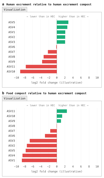
Figure 21:Diverging barplot illustrating differential abundance of features across sample categories. A common way to explore which features differ in their abundance across sample categories is with a diverging barplot. These generally focus on a reference group (Human Excrement Compost, or HEC, in this example) and compare another group to that. Here, Human Excrement (HE) is compared to HEC in panel a, and Food Compost is compared to HEC in panel b. The green bars highlight features that are present in higher abundance than in the reference group, while the red bars illustrate features that are present in lower abundance than in the reference group. Typically, these should be filtered by multiple-comparisons-corrected p-values (i.e., q-values). (Note: the results presented in this figure were not computed with ANCOM-BC2, unlike the data in the tutorial, because the constructed data set is too small for ANCOM-BC2 to be applied.)
Solution to Exercise 14
ASV c6c3ab4e828fb40d6e05967b7aac9338, an ASV classified to the Blautia_A genus, is most enriched in Human Excrement relative to HEC.
Its log fold change (LFC) was 1.84, and it was significantly different across HE and HEC with a q-value (q) of 0.04.
ASV 2e4f2b53b856c4def6d021d01f5abb70, an ASV classified to the species level as Dorea_A longicatena_B, is most depleted in Human Excrement relative to HEC.
Its LFC was -0.71, and it was not significantly different across HE and HEC (q=1).
ASV 8b5884acc8c736df09c4260b50dc9297, an ASV classified as Pseudomonas_E ovata, is most enriched in Food Compost relative to HEC.
Its LFC was 0.97, and it was not significantly different across HEC and Food Compost after multiple comparisons correction (p=0.04; q=1).
ASV e335f74033bc634af43ee6baa84fa247, an ASV classified as GCA-900066495 (a genus in the Firmicutes_A phylum), is most depleted in Food Compost relative to HEC.
Its LFC was -1.93, and it was significantly different across HEC and Food Compost with q=0.004.
Solution to Exercise 15
To collapse our ASVs into genera (i.e., level 6 of the GTDB version 202.0 taxonomy), we can use the following command.
qiime taxa collapse \
  --i-table asv-table-ms2-dominant-sample-types.qza \
  --i-taxonomy taxonomy.qza \
  --p-level 6 \
  --o-collapsed-table genus-table-ms2-dominant-sample-types.qza
genus_table_ms2_dominant_sample_types, = taxa_actions.collapse(
table=asv_table_ms2_dominant_sample_types,
taxonomy=taxonomy,
level=6,
)action_results <- taxa_actions$collapse(
table=asv_table_ms2_dominant_sample_types,
taxonomy=taxonomy,
level=6L,
)
genus_table_ms2_dominant_sample_types <- action_results$collapsed_tablegenus_table_ms2_dominant_sample_types, = use.action(
use.UsageAction(plugin_id='taxa',
action_id='collapse'),
use.UsageInputs(table=asv_table_ms2_dominant_sample_types,
taxonomy=taxonomy,
level=6),
use.UsageOutputNames(collapsed_table='genus_table_ms2_dominant_sample_types'))We can then provide the resulting table as the input to ANCOM-BC2.
qiime composition ancombc2 \
  --i-table genus-table-ms2-dominant-sample-types.qza \
  --m-metadata-file sample-metadata.tsv \
  --p-fixed-effects-formula SampleType \
  --p-reference-levels 'SampleType::Human Excrement Compost' \
  --o-ancombc2-output genus-ancombc2-results.qza
genus_ancombc2_results, = composition_actions.ancombc2(
table=genus_table_ms2_dominant_sample_types,
metadata=sample_metadata_md,
fixed_effects_formula='SampleType',
reference_levels=['SampleType::Human Excrement Compost'],
)action_results <- composition_actions$ancombc2(
table=genus_table_ms2_dominant_sample_types,
metadata=sample_metadata_md,
fixed_effects_formula='SampleType',
reference_levels=list('SampleType::Human Excrement Compost'),
)
genus_ancombc2_results <- action_results$ancombc2_outputgenus_ancombc2_results, = use.action(
use.UsageAction(plugin_id='composition',
action_id='ancombc2'),
use.UsageInputs(table=genus_table_ms2_dominant_sample_types,
metadata=sample_metadata,
fixed_effects_formula='SampleType',
reference_levels=['SampleType::Human Excrement Compost']),
use.UsageOutputNames(ancombc2_output='genus_ancombc2_results'))And finally, we can visualize the results. Notice that in this case, we’re not providing the taxonomy because we’ve already integrated that information by collapsing at the genus level.
qiime composition da-barplot \
  --i-data genus-ancombc2-results.qza \
  --o-visualization genus-ancombc2-barplot.qzv
genus_ancombc2_barplot_viz, = composition_actions.da_barplot(
data=genus_ancombc2_results,
)action_results <- composition_actions$da_barplot(
data=genus_ancombc2_results,
)
genus_ancombc2_barplot_viz <- action_results$visualizationuse.action(
use.UsageAction(plugin_id='composition',
action_id='da_barplot'),
use.UsageInputs(data=genus_ancombc2_results),
use.UsageOutputNames(visualization='genus-ancombc2-barplot'))In addition to the methods contained in the q2-composition plugin, new approaches for differential abundance testing are regularly introduced. It’s worth assessing the current state of the field when performing differential abundance testing to see if there are new methods that might be useful for your data.
Ensuring bioinformatics reproducibility and adapting the tutorial workflow for your own data
As a final step in the tutorial, we’re going to apply the rachis Provenance Replay functionality to the results that were just generated.
This will generate a script that documents the analysis steps that you ran, and in general this could be submitted as a detailed supplementary methods document with a paper presenting your results.
You can also use the resulting script to adapt the commands presented in this tutorial to your own data, adjusting parameter settings and metadata column headers as is relevant.
Change back to your home directory by running cd with no arguments (i.e., simply run: cd).
Assuming that you ran all of the steps above in a directory called gut-to-soil/, run the following command to generate a template script that you can adapt for your workflow:
qiime tools replay-provenance \
  --in-fp gut-to-soil/ \
  --recurse \
--out-fp g2s-replayed.bashSolution to Exercise 16
The trimming and truncation parameters used for DADA2 are indicated by the lines:
qiime dada2 denoise-paired \
  …
  --p-trunc-len-f 250 \
  --p-trunc-len-r 250 \
  --p-trim-left-f 0 \
  --p-trim-left-r 0 \
  …
The even sampling depth used when calling kmer-diversity is indicated by the lines:
qiime boots kmer-diversity \
  …
  --p-sampling-depth 96 \
  …
The confidence threshold used when calling classify-sklearn is indicated by the lines:
qiime feature-classifier classify-sklearn \
  …
  --p-confidence 0.7 \
  …
The qiime tools import and qiime demux subsample-paired commands were not run in this tutorial.
Rather, they were data preparation steps that someone else ran prior to this tutorial.
Because they are in data provenance, it’s still possible to know exactly what those commands were and how they could be re-run.
Solution to Exercise 17
rachis-view includes information on the run time of jobs, and the software and software versions that were installed in the environment when the command was run.
Provenance Replay presents commands formatted for re-running as a script.
Importantly, neither contains input or output file names.
rachis doesn’t track that information because it’s not stable.
For example, a file can be renamed after it is created, which means that a file name (if saved in provenance) would be out of date.
Instead, every rachis Result is assigned a UUID which cannot be changed without invalidating the Result.
You can find a Result’s UUID in rachis-view.
Conclusion
In this tutorial we presented a reproducible workflow and supporting data for applying amplicon sequencing and bioinformatics tools to study HEC. This workflow offers insight into the typical steps in an amplicon-sequencing-based microbiome analysis. The outcomes presented here are those that are most common to all amplicon analysis workflows, and from this point, analysis tends to diverge to focus on study-specific questions. The QIIME 2 documentation covers an increasingly broad selection of these analyses, and our developer and support community is available to advise as needed. To explore some of the more study-specific analyses with the tutorial data presented here, a few next steps could be:
Build a machine learning classifier that classifies samples according to the three dominant sample types in the feature table that we used with ANCOM-BC2. (Hint: see
classify-samplesin the q2-sample-classifier plugin Bokulich et al., 2018.)Perform a longitudinal analysis that tracks which taxa change most with time in different buckets. (Hint: see
feature-volatilityusing the q2-longitudinal plugin Bokulich et al., 2018).Identify a more modern taxonomy classifier using the resources described earlier and apply it to the tutorial data. How does it change the taxonomic assignments? (Here’s a hint on how to compare taxonomic annotations obtained from different classifiers.)
The full dataset (five sequencing runs) is available in the gut-to-soil Artifact Repository Caporaso & Meilander, 2025. Download one of the larger sequencing runs (we worked with a small sequencing run that was generated as a preliminary test), and adapt the commands in the provenance replay script to analyze a bigger dataset.
The
rachisdevelopers provide a utility, artifinder, designed to help you find and identify Artifacts that are relevant to your analysis from a directory that might contain a mix of relevant and irrelevant Artifacts and Visualizations. Install this, and try it out by following the instructions in the artifinder documentation.rachisrecently enabled the generation of Reports, which allow for integration of multiple.qzvs into one, for easy sharing with colleagues, in manuscripts, and elsewhere. Create a report from all of the.qzvs that you generated using the following command. Then, curate a more specific one that you think presents the most relevant information and interesting results from the tutorial analysis. Experiment with customizing your report in Python, as illustrated in this example.qiime tools make-report --report-path gut-to-soil-visualizations.qzv \ $(find gut-to-soil/ -name '.*' -prune -o -name '*.qzv' -print)
Now that you’ve completed this tutorial, you should be able to adapt the commands presented here to perform your own microbiome marker gene data analysis.
You can find additional information and learning materials in our documentation starting from the rachis-library, and if you need additional guidance the QIIME 2 Forum is an excellent resource containing over 10 years of questions and answers related to QIIME 2 and microbiome data science.
Thanks for your interest, and we hope to see you on the QIIME 2 Forum!
A final word on why we chose this tutorial data
A final word on the data used in this tutorial: broader adoption of HEC as a waste management strategy would offer wide-ranging benefits, including for fresh water conservation, reduction of environmental contamination, improvement of public health nearly everywhere on Earth, and the advancement of the technologies that will someday enable human settlement off-Earth. Microbiomes drive the HEC reaction, and we postulate that HEC microbiome science and engineering can help optimize composting conditions for efficiency and safety, support bioprospecting for thermostable biotechnologically relevant enzymes (such as those that can degrade problematic waste materials), and inform accessible protocols for ensuring stringent safety standards are consistently met.
Additionally, we think these data are great for learning. They embody highly dynamic microbiomes which consistently change from compositions associated with the human microbiome to those that look more like soil microbiomes. As a result, we hope that regardless of where your interests lie in microbiome science, the techniques and the microbes represented here will be relevant to your work.
As you start your journey in microbiome science we urge you to keep HEC systems in mind. Broader adoption of HEC technology isn’t something we envision happening quickly or universally, but because of the scale of the problems, even small advances can have far-reaching impacts. If you’re interested in HEC-related problems and solutions, feel free to connect with us through the Compost Microbiome Lab (CML 🐪). Find a longer discussion of this here.
The two non-default parameters passed to
fit-classifier-naive-bayeshere arefeat_ext__n_features(default 8192) andclassify__chunk_size(default 20000).feat_ext__n_featuressets the size of the hashed k-mer feature space: every 7-mer in a reference sequence is hashed into one of this many buckets, so a smaller value means more distinct k-mers share a bucket and the classifier has less information to separate similar taxa.classify__chunk_sizesets how many reference sequences are passed to the classifier at a time during training; each chunk is expanded into a dense sequences × classes label matrix, so this controls a transient memory peak during training.chunk_sizehas no effect on the resulting classifier: models trained with different chunk sizes are identical.n_featuresdoes affect the classifier. With this reference, reducing it from 8192 to 2048 roughly halves the memory needed to train and to run the classifier, but on the sequences in this tutorial it also reduces the number of ASVs classified to genus level by about a quarter and to species level by about half; the assignments that are made agree with the default classifier’s, so the cost is resolution rather than error. When training your own classifier, leave both parameters at their defaults unless you run out of memory. If you do, note that reducingchunk_sizealone made little difference to peak memory in our testing; the memory saving comes mainly fromn_features, and the two together reduce it further. Reducing the number of classes (for example, by collapsing the reference taxonomy to genus level withrescript edit-taxonomy) or using a pre-trained classifier from the QIIME 2 Library are alternatives that avoid this trade-off. This footnote text, the parameter modifications made for classifier training in the tutorial, and the analyses described here were prepared with AI assistance.kmerization of biological sequences is described in the Database Searching chapter of An Introduction to Applied Bioinformatics.
Learn more about the available metrics in this QIIME 2 Forum post.
This process is discussed in the Machine Learning in Bioinformatics chapter of An Introduction to Applied Bioinformatics.